6.1: Introduction to Phasors

We will not always be dealing with transmission lines excited with a pulse. Although this is a good model for digital circuitry, it will not always apply. When we go to analog signals (rf, high frequency analog, etc.) we will need more tools than are available to us at this point. In the not-too-distant-past, the material we will next consider was starting to be considered passé. The rf spectrum was more or less filled up, and the watchword was "digital". Now, in the new age of wireless communication, cell phones, and rf Local Area Networks, demand for engineers who understand ac behavior on transmission lines and who can design systems which work well with rf signals are very much in demand. Pay heed to what we say here, and you might well find yourself with many lucrative job offers in the future.

To begin, we want to consider a transmission line which is being excited with an oscillating source, as in Figure \(\PageIndex{1}\).

Figure \(\PageIndex{1}\): Sinusoidal excitation of a loaded transmission line

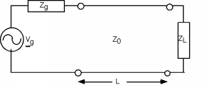
The usual set-up includes a source, with a sinusoidal output, a source impedance \(Z_{g}\), a transmission line with impedance \(Z_{0}\), length \(L\) meters, and a load of impedance \(Z_{L}\) at the end.

Let's look at the source first. We can describe the output waveform from the generator as \[V(t) = V_{g} \cos (\omega t + \theta)\]

When plotted, this looks like Figure \(\PageIndex{2}\).

Figure \(\PageIndex{2}\): Excitation waveform

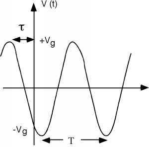
The oscillating waveform has a period \(T\) and its angular frequency \(\omega\) is given as \[\begin{array}{l} \omega &=& \dfrac{2 \pi}{T} \\ &=& 2 \pi f \end{array}\]

The angle \(\theta\), which specifies how much the wave is leading a cosine function with zero off-set, is given by \[\theta = 2 \pi \frac{\tau}{T}\]

What we do not want to do is carry a bunch of sine and cosine functions around with us everywhere. Once we start multiplying and dividing, the trig turns into a big mess, and gets in the way of our understanding of what is going on. The way we deal with this is to introduce phasors.

Since we know from Euler's Identity \[V_{g} e^{i(\omega t + \theta)} = V_{g} (\cos (\omega t + \theta) + i \sin (\omega t + \theta))\]

if we take a real part of \(V_{g} e^{i (\omega t + \theta)}\), we will extract the voltage waveform we desire. We will re-write this function as \[V_{g} e^{i (\omega t + \theta)} = V_{g} e^{i \omega} e^{i \omega t}\]

and then define \(\tilde{V}_{g}\) as the phasor voltage where \[\tilde{V}_{g} = V_{g} e^{i \theta}\]

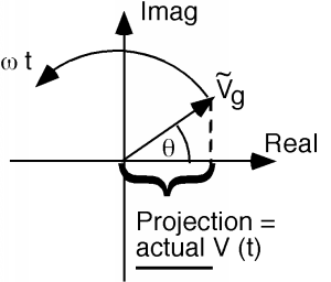
Note that \(\tilde{V}_{g}\) is a complex quantity, with both a magnitude \(\left| V_{g} \right|\) and a phase angle \(\theta\). In order to retrieve a real voltage signal from a phasor, we have to multiply the phasor by \(e^{i \omega t}\) and then take the real part. Note that this is the same thing as plotting the phasor on the complex plane, and then observing the projection of the phasor on the real axis, as the phasor rotates around at a rate \(\omega t\) as shown in Figure \(\PageIndex{3}\).

Figure \(\PageIndex{3}\): Phasor representation

This method of visualization will sometimes help make results seem a little easier to understand, or at least check for reasonableness.