6.2: A/C Line Behavior

Last updated
Save as PDF

Page ID: 88574

$ \newcommand{\vecs}[1]{\overset { \scriptstyle \rightharpoonup} {\mathbf{#1}} } $ $ \newcommand{\vecd}[1]{\overset{-\!-\!\rightharpoonup}{\vphantom{a}\smash {#1}}} $$\newcommand{\id}{\mathrm{id}}$ $ \newcommand{\Span}{\mathrm{span}}$ $ \newcommand{\kernel}{\mathrm{null}\,}$ $ \newcommand{\range}{\mathrm{range}\,}$ $ \newcommand{\RealPart}{\mathrm{Re}}$ $ \newcommand{\ImaginaryPart}{\mathrm{Im}}$ $ \newcommand{\Argument}{\mathrm{Arg}}$ $ \newcommand{\norm}[1]{\| #1 \|}$ $ \newcommand{\inner}[2]{\langle #1, #2 \rangle}$ $ \newcommand{\Span}{\mathrm{span}}$ $\newcommand{\id}{\mathrm{id}}$ $ \newcommand{\Span}{\mathrm{span}}$ $ \newcommand{\kernel}{\mathrm{null}\,}$ $ \newcommand{\range}{\mathrm{range}\,}$ $ \newcommand{\RealPart}{\mathrm{Re}}$ $ \newcommand{\ImaginaryPart}{\mathrm{Im}}$ $ \newcommand{\Argument}{\mathrm{Arg}}$ $ \newcommand{\norm}[1]{\| #1 \|}$ $ \newcommand{\inner}[2]{\langle #1, #2 \rangle}$ $ \newcommand{\Span}{\mathrm{span}}$$\newcommand{\AA}{\unicode[.8,0]{x212B}}$

If we are going to try to use phasors on a transmission line, then we have to allow for spatial variation as well. This is simple to do, if we just let the phasor be a function of $x$, so we have $\widetilde{V} (x)$. How the phasor varies in $x$ is one of the things we now have to find out.

Let's start with the Telegrapher's Equations again. \[\frac{\partial V(x, t)}{\partial x} = (- \mathbf{L}) \frac{\partial I(x, t)}{\partial t}\] \[\frac{\partial I(x, t)}{\partial x} = (- \mathbf{C}) \frac{\partial V(x, t)}{\partial t}\]

For $V(x, t)$ we can now substitute $\widetilde{V} (x) e^{i \omega t}$ and for $I(x, t)$ we plug in $\widetilde{I} (x) e^{i \omega t}$. So we get: \[\frac{\partial \left( \widetilde{V}(x) e^{i \omega t} \right)}{\partial x} = (- \mathbf{L}) \frac{\partial \left( \widetilde{I}(x) e^{i \omega t} \right)}{\partial t}\]

and \[\frac{\partial \left(\widetilde{I}(x) e^{i \omega t} \right)}{\partial x} = (- \mathbf{C}) \frac{\partial \left(\widetilde{V}(x) e^{i \omega t} \right)}{\partial t}\]

We take the derivative with respect to time, which brings down an $i \omega$, and then we cancel the $i \omega$ from both sides of each equation: \[\frac{\partial \widetilde{V}(x)}{\partial x} = -\left(i \omega \mathbf{L} \widetilde{I}(x) \right)\]

and \[\frac{\partial \widetilde{I}(x)}{\partial x} = -\left(i \omega \mathbf{C} \tilde{V}(x) \right)\]

Voila! In one simple motion, we have completely eliminated the time variable, $t$, from our equations! It is not really gone, of course, for once we figure out what $\widetilde{V} (x)$ is, we have to multiply it by $e^{i \omega t}$ and then take the real part before we can extract, once again, the actual $V(x, t)$ that we want. Nonetheless, insofar as the telegrapher's equations are concerned, $t$ has disappeared from the radar screen.

To solve these we do just what we did with the transient problem. We take a derivative with respect to $x$ of Equation $\PageIndex{5}$, which gives us a $\frac{\partial \widetilde{I} (x)}{\partial x}$ on the right hand side, for which we can substitute Equation $\PageIndex{6}$, which leaves us with \[\frac{\partial^{2} \widetilde{V} (x)}{\partial x^{2}} = - \left(\omega^{2} \mathbf{LC} \widetilde{V} (x)\right)\]

($-$ times $-$ is $+$, but $ii = -1$ and so we have a $-$ in front of the $\omega^{2}$). We then re-write Equation $\PageIndex{7}$ as \[\frac{\partial^{2} \widetilde{V} (x)}{\partial x^{2}} + \omega^{2} \mathbf{LC} \widetilde{V} (x) = 0\]

The simplest solution to this equation is \[\widetilde{V} (x) = V_{0} e^{\pm \left(i \omega \sqrt{\mathbf{LC}} x \right)}\]

from which we can then get the actual voltage signal \[\begin{array}{l} V(x, t) &=& \widetilde{V}(x) e^{i \omega t} \\[4pt] &=& V_{0} e^{i \left(\omega t \pm \omega \sqrt{\mathbf{LC}} x \right)} \end{array}\]

Note that we could factor out an $e^{i \omega \sqrt{\mathbf{LC}}}$ from the exponent, which, since it is just a constant, we could include in $V_{0}$ (and call it $V_{0}'$), switch the order of $x$ and $t$, and write Equation $\PageIndex{10}$ as \[V(x, t) = V_{0}' e^{i \left(x \pm \frac{1}{\sqrt{\mathbf{LC}}} t \right)}\]

which looks a lot like the "general" $f(x \pm vt)$ solution we were talking about earlier!

The number $\omega \sqrt{\mathbf{LC}}$ is special. It is usually represented with the Greek letter $\beta$ and is called the propagation coefficient. Thus we have \[V(x, t) = V_{0} e^{i \left(\omega t \pm \beta x\right)}\]

As previously, a point on the wave of constant phase requires that the argument inside the parenthesis remains constant. Thus if $V(x_{1}, t_{1})$ is going to equal $V(x_{2}, t_{2})$ (i.e., what was at point $x_{1}$ at $t_{1}$ is now at $x_{2}$ at time $t_{2}$), it must be that \[\omega t_{1} \pm \beta x_{1} = \omega t_{2} \pm \beta x_{2}\]

\frac{x_{2} - x_{1}}{t_{2} - t_{1}} = \frac{Δ}{(x)} = \pm (\frac{ω}{β}) = \pm (\frac{ω}{ω}) = \pm (\frac{1}{\sqrt{L C}}) \equiv v_{p}

Which one again, defines the phase velocity of the wave. Other relationships to keep in mind are

β = \frac{2}{π}

\begin{array}{rcl} λ & = & \frac{v_{p}}{f} \\ = & \frac{\frac{ω}{β}}{\frac{ω}{2}} \\ = & \frac{2}{π} \end{array}

The first comes from the fact that the wave varies in $x$ as $e^{i β x}$ . Thus when $x = γ$ , the wavelength, $β γ$ just increases by $2 π$ , to get the phasor to go through one full rotation. Note also, as before, the choice of the minus sign in the ± in Equation represents a wave going in the $x$ direction, while the choice of the + sign will give a wave going in the $- x$ direction. Clearly, by starting out taking the x-derivative of the equation for $I (x, t)$ we would end up with

I (x, t) = I_{0} e^{i (ω t \pm β x)}

Let's consider the two phasors then, and define the voltage phasor associated with the positive going voltage wave as

{\tilde{V}}_{plus} (x) = V^{+} e^{- (i β x)}

and the negative voltage phasor as

{\tilde{V}}_{minus} (x) = V^{-} e^{i β x}

We should keep in mind that both $V^{+}$ and $V^{-}$ can be, and probably are, complex numbers. (From now on we will drop the little ~ over the variables because its very tedious to get it to show up with this word processor. You will just have to keep in mind that any variable we do not explicitly put inside absolute value markers (i.e. $| V^{+} |$ ) is going to be, in general, a complex number). We will, of course, have similar expressions for the positive and negative going current waves.

Let's consider the positive going current and voltage waves, and plug them into Equation.

\frac{\partial^{} (V^{+} e^{- (i β x)})}{\partial x^{}} = - (i ω L I^{+} e^{- (i β x)})

The x-derivative brings down a $- (i β)$ , the $e^{- (i β x)}$ 's cancel, and we have

V^{+} = \frac{i ω L}{i β} I^{+}

But, since $β = ω \sqrt{L C}$ we have

V^{+} = \sqrt{\frac{L}{C}} I^{+} \equiv Z_{0} I^{+}

as we had before.

So, what has changed? Not much from the case of transients on a line. We will now assume we have a steady state problem. This means we turned on the generator a long time ago. We assume that it has been connected to the line long enough so that all transient behavior has died away, and that voltages and currents are not changing any more (except oscillating at frequency $ω$ , of course).

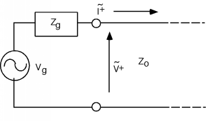
If the line is semi-infinite (or matched with a load equal to $Z_{0}$ ) as in Figure $\PageIndex{1}$ then it is pretty obvious that

V^{+} = \frac{Z_{0}}{Z_{0} + Z_{g}} V_{g}

where $Z_{g}$ is the source impedance, and $V_{g}$ is the source voltage phasor.

A transmission line with impedance Z_0 and infinite length is attached at its left end to a sinusoidal voltage source v_g with a source impedance z_g. The voltage from the lower to the upper left end of the transmission line is tilde V+, and the current entering the transmission line, moving to the right, is tilde I+. — Figure $\PageIndex{1}$: A Wave On a Semi-Infinite Line