2.2: Two-Port Networks

Many of the techniques employed in analyzing circuits require that the voltage at each terminal of a circuit be referenced to a common point such as ground. In microwave circuits it is generally difficult to do this. Recall that with transmission lines it is not possible to establish a common ground point. However, with transmission lines (and circuit elements that utilize distributed effects) it was seen that for each signal current there is a signal return current. Thus at radio frequencies, and for circuits that are distributed, ports are used, as shown in Figure 2.1.1(a), which define the voltages and currents for what is known as a two-port network, or just two-port.\(^{1}\) The network in Figure 2.1.1(a) has four terminals and two ports. A port voltage is defined as the voltage difference between a pair of terminals with one of the terminals in the pair becoming the reference terminal. The current entering the network at the top terminal of Port \(\mathsf{1}\) is \(I_{1}\) and there is an equal current leaving the reference terminal. This arrangement clearly makes sense when transmission lines are attached to Ports \(\mathsf{1}\) and \(\mathsf{2}\), as in Figure 2.1.1(b). With transmission lines at Ports \(\mathsf{1}\) and \(\mathsf{2}\) there will be traveling-wave voltages, and at the ports the traveling-wave components add to give the total port voltage. In dealing with nondistributed circuits it is preferable to use the total port voltages and currents—\(V_{1},\: I_{1},\: V_{2},\) and \(I_{2}\), shown in Figure 2.1.1(a). However, with distributed elements it is preferable to deal with traveling voltages and currents—\(V_{1}^{+},\: V_{1}^{−},\: V_{2}^{+},\) and \(V_{2}^{−}\), shown in Figure 2.1.1(b). RF and microwave design necessarily requires switching between the two forms.

2.1.1 Reciprocity, Symmetry, Passivity, and Linearity

Reciprocity, symmetry, passivity, and linearity are fundamental properties of networks. A network is linear if the response (voltages and currents) is linearly dependent on the drive level, and superposition also applies. So if the two-port shown in Figure 2.1.1(a) is linear, the currents \(I_{1}\) and \(I_{2}\) are linear functions of \(V_{1}\) and \(V_{2}\). An example of a linear network would be one with resistors and capacitors. A network with a diode would be an example of a nonlinear network.

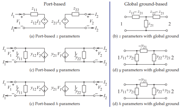
Figure \(\PageIndex{1}\): The \(z-,\: y-,\) and \(h-\) parameter equivalent circuits for port-based and global ground representations. The immittances are shown as impedances.

A passive network has no internal sources of power and so a network with an embedded battery is not a passive network. A symmetrical two-port has the same characteristics at each of the ports. An example of a symmetrical network is a transmission line with a uniform cross section.

A reciprocal two-port has a response at Port \(\mathsf{2}\) from an excitation at Port \(\mathsf{1}\) that is the same as the response at Port \(\mathsf{1}\) to the same excitation at Port \(\mathsf{2}\). As an example, consider the two-port in Figure 2.1.1(a) with \(V_{2} = 0\). If the network is reciprocal, then the ratio \(I_{2}/V_{1}\) with \(V_{2} = 0\) will be the same as the ratio \(I_{1}/V_{2}\) with \(V_{1} = 0\). Most networks with resistors, capacitors, and transmission lines, for example, are reciprocal. A transistor amplifier is not reciprocal, as gain, analogous to the ratio \(V_{2}/V_{1}\), is in just one direction (or unidirectional).

2.2.2 Parameters Based on Total Voltage and Current

Here port-based impedance \((z)\), admittance \((y)\), and hybrid \((h)\) parameters will be described. These are similar to the more conventional \(z,\: y,\) and \(h\) parameters defined with respect to a common or global ground. The contrasting circuit representations of the parameters are shown in Figure \(\PageIndex{1}\).

Impedance parameters

First, port-based impedance parameters will be considered based on total port voltages and currents as defined for the two-port in Figure 2.1.1. These parameters are also referred to as port impedance parameters or just impedance parameters when the context is understood to be ports.

Port-based impedance parameters, or \(z\) parameters, are defined as

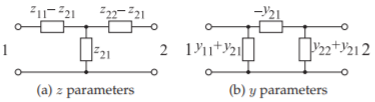
Figure \(\PageIndex{2}\): Circuit equivalence of the \(z\) and \(y\) parameters for a reciprocal network (in (b) the elements are admittances).

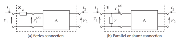
Figure \(\PageIndex{3}\): Connection of a two-terminal element to a two-port.

\[\begin{align}\label{eq:1}V_{1}&=z_{11}I_{1}+z_{12}I_{2} \\ \label{eq:2}V_{2}&=z_{21}I_{1}+z_{22}I_{2}\end{align} \]

or in matrix form as

\[\label{eq:3}\mathbf{V}=\mathbf{ZI} \]

The double subscript on a parameter is ordered so that the first refers to the output and the second refers to the input, so \(z_{ij}\) relates the voltage output at Port \(i\) to the current input at Port \(j\). If the network is reciprocal, then \(z_{12} = z_{21}\), but this simple type of relationship does not apply to all network parameters. The reciprocal circuit equivalence of the \(z\) parameters is shown in Figure \(\PageIndex{2}\)(a). It will be seen that the \(z\) parameters are convenient parameters to use when an element is in series with one of the ports, as then the operation required in developing the \(z\) parameters of the larger network is just addition.

Figure \(\PageIndex{3}\)(a) shows the series connection of a two-terminal element with a two-port designated as network \(\text{A}\). The \(z\) parameters of network \(\text{A}\) are

\[\label{eq:4}\mathbf{Z}_{A}=\left[\begin{array}{cc}{z_{11}^{(A)}}&{z_{12}^{(A)}}\\{z_{21}^{(A)}}&{z_{22}^{(A)}}\end{array}\right] \]

so that

\[\begin{align}\label{eq:5} V_{1}^{(A)}&= z_{11}^{(A)}I_{1} + z_{12}^{(A)}I_{2} \\ \label{eq:6} V_{2}&= z_{21}^{(A)}I_{1} + z_{22}^{(A)}I_{2} \end{align} \]

Now

\[\label{eq:7} V_{1} = zI_{1} + V_{1}^{(A)} = zI_{1} + z_{11}^{(A)}I_{1} + z_{12}^{(A)}I_{2} \]

so the \(z\) parameters of the whole network can be written as

\[\label{eq:8}\mathbf{Z}=\left[\begin{array}{cc}{z}&{0}\\{0}&{0}\end{array}\right]+\mathbf{Z}_{A} \]

Example \(\PageIndex{1}\): Thevenin equivalent of a source with a two-port

What is the Thevenin equivalent circuit of the source-terminated two-port network on the right.

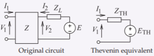
Figure \(\PageIndex{4}\)

Solution

From the original circuit

\[\begin{align}\label{eq:9}V_{1}&=Z_{11}I_{1}+Z_{12}I_{2} \\ \label{eq:10}V_{2}&=Z_{21}I_{1}+Z_{22}I_{2} \\ \label{eq:11}V_{2}&=E-I_{2}Z_{L}\end{align} \]

Substituting Equation \(\eqref{eq:11}\) in Equation \(\eqref{eq:10}\)

\[\label{eq:12}E=Z_{21}I_{1}+(Z_{22}+Z_{L})I_{2} \]

Multiplying Equation \(\eqref{eq:9}\) by \((Z_{22} + Z_{L})\) and Equation \(\eqref{eq:12}\) by \(Z_{12}\)

\[\begin{align} (Z_{22} + Z_{L})V_{1} &= (Z_{22} + Z_{L})Z_{11}I_{1}\nonumber \\ \label{eq:13}&\quad +(Z_{22} + Z_{L})Z_{12}I_{2} \\ \label{eq:14} Z_{12}E &= Z_{12}Z_{21}I_{1} + Z_{12}(Z_{22} + Z_{L})I_{2}\end{align} \]

Subtracting Equation \(\eqref{eq:14}\) from Equation \(\eqref{eq:13}\)

\[(Z_{22} + Z_{L})V_{1} − Z_{12}E = [(Z_{22} + Z_{L})Z_{11}−]I_{1}\nonumber \]

\[\label{eq:15}V_{1}=\frac{Z_{12}E}{Z_{22}+Z_{L}}+\left(Z_{11}-\frac{Z_{12}Z_{21}}{Z_{22}+Z_{L}}\right)I_{1} \]

For the Thevenin equivalent circuit \(V_{1} = E_{\text{TH}} + I_{1}Z_{\text{TH}}\) and so

\[\label{eq:16}Z_{\text{TH}}=\left(Z_{11}-\frac{Z_{12}Z_{21}}{Z_{22}+Z_{L}}\right)\quad\text{and}\quad E_{\text{TH}}=\frac{Z_{12}E}{Z_{22}+Z_{L}} \]

Admittance parameters

When an element is in shunt with a two-port, port-based admittance parameters, or \(y\) parameters, are the most convenient to use. These are defined as

\[\begin{align}\label{eq:17}I_{1}&=y_{11}V_{1}+y_{12}V_{2} \\ \label{eq:18}I_{2}&=y_{21}V_{1}+y_{22}V_{2}\end{align} \]

or in matrix form as

\[\label{eq:19}\mathbf{I}=\mathbf{YV} \]

Now, for reciprocity, \(y_{12} = y_{21}\) and the circuit equivalence of the \(y\) parameters is shown in Figure \(\PageIndex{2}\)(b). Consider the shunt connection of an element shown in Figure \(\PageIndex{3}\)(b) where the \(y\) parameters of network \(\text{A}\) are

\[\label{eq:20}\mathbf{Y}_{A}=\left[\begin{array}{cc}{y_{11}^{(A)}}&{y_{12}^{(A)}}\\{y_{21}^{(A)}}&{y_{22}^{(A)}}\end{array}\right]=\mathbf{Z}_{A}^{-1} \]

The port voltages and currents are related as follows

\[\begin{align} \label{eq:21} I_{1}^{(A)} &= y_{11}^{(A)}V_{1} + y_{12}^{(A)}V_{2}\quad\text{ and }\quad I_{2} = y_{21}^{(A)}V_{1} + y_{22}^{(A)}V_{2} \\ \label{eq:22}I_{1} &= yV_{1} + I_{1}^{(A)}= (y + y_{11}^{(A)})V_{1} + y_{12}^{(A)}V_{2} \end{align} \]

Thus the \(y\) parameters of the whole network are

\[\label{eq:23}\mathbf{Y}=\left[\begin{array}{cc}{y}&{0}\\{0}&{0}\end{array}\right]+\mathbf{Y}_{A} \]

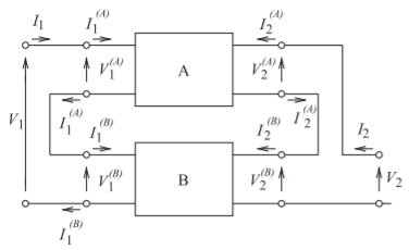
Figure \(\PageIndex{5}\): Series connection of two two-port networks.

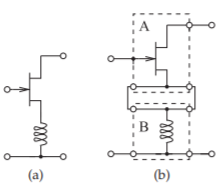
Figure \(\PageIndex{6}\): Example of a series connection of two-port networks: (a) an amplifier; and (b) its components represented as two-port networks.

Hybrid parameters

Sometimes it is more convenient to use hybrid parameters, or \(h\) parameters, defined by

\[\label{eq:24}V_{1} = h_{11}I_{1} + h_{12}V_{2}\quad\text{ and }\quad I_{2} = h_{21}I_{1} + h_{22}V_{2} \]

or in matrix form as

\[\label{eq:25}\left[\begin{array}{c}{V_{1}}\\{I_{2}}\end{array}\right]=\mathbf{H}\left[\begin{array}{c}{I_{1}}\\{V_{2}}\end{array}\right] \]

These parameters are convenient to use with transistor circuits, as they describe a voltage-controlled current source that is a simple model of a transistor.

The choice of which network parameters to use depends on convenience, but as will be seen throughout this text, some parameters naturally describe a particular characteristic desired in a design. For example, with Port \(\mathsf{1}\) being the input port of an amplifier and Port \(\mathsf{2}\) being the output port, \(h_{21}\) describes the current gain of the amplifier.

2.2.3 Series Connection of Two-Port Networks

A series connection of two two-ports is shown in Figure \(\PageIndex{5}\). An example of when the series connection occurs is shown in Figure \(\PageIndex{6}\), which is the schematic of a transistor amplifier configuration with an inductor in the source leg. The transistor and the inductor can each be represented as two-ports so that the circuit of Figure \(\PageIndex{6}\)(a) is the series connection of two two-ports, as shown in Figure \(\PageIndex{6}\)(b). In the following, two-port parameters of the complete circuit are developed using the two-port parameter descriptions of the component two-ports. The procedure with any interconnection is to write down the relationships between the voltages and currents of the constituent networks. Which network parameters to use requires identification of the arithmetic path requiring the fewest operations.

Simple algebra relates the various total voltage and current parameters. From Figure \(\PageIndex{5}\),

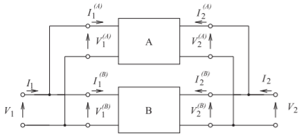
Figure \(\PageIndex{7}\): Parallel connection of two-port networks.

\[I_{1}^{(A)}= I_{1}^{(B)} = I_{1},\quad I_{2}^{(A)} = I_{2}^{(B)}= I_{2},\quad V_{1} = V_{1}^{(A)}+ V_{1}^{(B)},\quad V_{2} = V_{2}^{(A)}+ V_{2}^{(B)} \nonumber \]

which in matrix form becomes

\[\label{eq:26}\left[\begin{array}{c}{V_{1}^{(A)}}\\{V_{2}^{(A)}}\end{array}\right] = \left[\begin{array}{cc}{z_{11}^{(A)}}&{z_{12}^{(A)}}\\{z_{21}^{(A)}}&{z_{22}^{(A)}}\end{array}\right] \left[\begin{array}{c}{I_{1}^{(A)}}\\{I_{2}^{(A)}}\end{array}\right];\: \left[\begin{array}{c}{V_{1}^{(B)}}\\{V_{2}^{(B)}}\end{array}\right] =\left[\begin{array}{cc}{z_{11}^{(B)}}&{z_{12}^{(B)}}\\{z_{21}^{(B)}}&{z_{22}^{(B)}}\end{array}\right] \left[\begin{array}{c}{I_{1}^{(B)}}\\{I_{2}^{(B)}}\end{array}\right] \]

or

\[\label{eq:27}\left[\begin{array}{c}{V_{1}}\\{V_{2}}\end{array}\right]=(\mathbf{Z}^{A}+\mathbf{Z}^{B})\left[\begin{array}{c}{I_{1}}\\{I_{2}}\end{array}\right] \]

Thus the impedance matrix of the series connection of two-ports is

\[\label{eq:28}\mathbf{Z}=\mathbf{Z}_{\mathbf{A}}+\mathbf{Z}_{\mathbf{B}} \]

2.2.4 Parallel Connection of Two-Port Networks

Admittance parameters are most conveniently combined to obtain the overall parameters of the two-port parallel connection of Figure \(\PageIndex{7}\). The total voltage and current are related by

\[\begin{align}\label{eq:29}V_{1}^{(A)}&=V_{1}^{(B)}=V_{1} \\ \label{eq:30}V_{2}^{(A)}&=V_{2}^{(B)}=V_{2} \\ \label{eq:31} I_{1}&=I_{1}^{(A)}+I_{1}^{(B)} \\ \label{eq:32} I_{2}&=I_{2}^{(A)}+I_{2}^{(B)}\end{align} \]

and

\[\begin{align}\label{eq:33}\left[\begin{array}{c}{I_{1}^{(A)}}\\{I_{2}^{(A)}}\end{array}\right]&=\left[\begin{array}{cc}{y_{11}^{(A)}}&{y_{12}^{(A)}}\\{y_{21}^{(A)}}&{y_{22}^{(A)}}\end{array}\right]\left[\begin{array}{c}{V_{1}^{(A)}}\\{V_{2}^{(A)}}\end{array}\right] \\ \label{eq:34} \left[\begin{array}{c}{I_{1}^{(B)}}\\{I_{2}^{(B)}}\end{array}\right]&=\left[\begin{array}{cc}{y_{11}^{(B)}}&{y_{12}^{(B)}}\\{y_{21}^{(B)}}&{y_{22}^{(B)}}\end{array}\right]\left[\begin{array}{c}{V_{1}^{(B)}}\\{V_{2}^{(B)}}\end{array}\right]\end{align} \]

So the overall \(y\) parameter relation is

\[\label{eq:35}\left[\begin{array}{c}{I_{1}}\\{I_{2}}\end{array}\right]=(\mathbf{Y}_{A}+\mathbf{Y}_{B})\left[\begin{array}{c}{V_{1}}\\{V_{2}}\end{array}\right] \]

Figure \(\PageIndex{8}\) is an example of subcircuits that can be represented as two-ports that are then connected in parallel.

2.2.5 Series-Parallel Connection of Two-Port Networks

A similar approach to that in the preceding subsection is followed in developing the overall network parameters of the series-parallel connection of

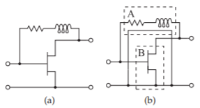
Figure \(\PageIndex{8}\): Example of the parallel connection of two two-ports: (a) a feedback amplifier; and (b) its components represented as two-port networks \(\text{A}\) and \(\text{B}\).

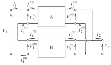
Figure \(\PageIndex{9}\): Series-parallel connection of two-ports.

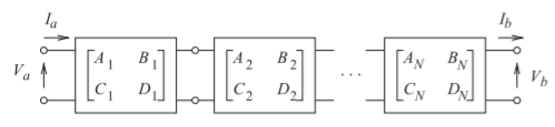
Figure \(\PageIndex{10}\): Cascade of two-port networks.

two-ports shown in Figure \(\PageIndex{9}\). Now,

\[\begin{align}\label{eq:36} I_{1}^{(A)}&=I_{1}^{(B)}=I_{1} \\ \label{eq:37}V_{2}^{(A)}&=V_{2}^{(B)}=V_{2} \\ \label{eq:38}V_{1}&=V_{1}^{(A)}+V_{1}^{(B)} \\ \label{eq:39} I_{2}&=I_{2}^{(A)}+I_{2}^{(B)}\end{align} \]

and so, using hybrid parameters,

\[\begin{align}\label{eq:40}\left[\begin{array}{c}{V_{1}^{(A)}}\\{I_{2}^{(A)}}\end{array}\right]&=\left[\begin{array}{cc}{h_{11}^{(A)}}&{h_{12}^{(A)}} \\ {h_{21}^{(A)}} &{h_{22}^{(A)}}\end{array}\right]\left[\begin{array}{c}{I_{1}^{(A)}}\\{V_{2}^{(A)}}\end{array}\right] \\ \label{eq:41} \left[\begin{array}{c}{V_{1}^{(B)}}\\{I_{2}^{(B)}}\end{array}\right]&=\left[\begin{array}{cc}{h_{11}^{(B)}}&{h_{12}^{(B)}} \\ {h_{21}^{(B)}} &{h_{22}^{(B)}}\end{array}\right]\left[\begin{array}{c}{I_{1}^{(B)}}\\{V_{2}^{(B)}}\end{array}\right] \end{align} \]

Putting this in compact form:

\[\label{eq:42}\left[\begin{array}{c}{V_{1}}\\{I_{2}}\end{array}\right]=(\mathbf{H}_{A}+\mathbf{H}_{B})\left[\begin{array}{c}{I_{1}}\\{V_{2}}\end{array}\right] \]

2.2.6 \(ABCD\) Matrix Characterization of Two-Port Networks

\(ABCD\) parameters are the best parameters to use when cascading two-ports, as in Figure \(\PageIndex{10}\), and total voltage and current relationships are required. First, consider Figure \(\PageIndex{11}\), which puts the voltages and currents

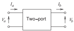
Figure \(\PageIndex{11}\): Two-port network with cascadable voltage and current definitions.

in cascadable form with the input variables in terms of the output variables:

\[\label{eq:43}\left[\begin{array}{c}{V_{a}}\\{I_{a}}\end{array}\right]=\left[\begin{array}{cc}{A}&{B}\\{C}&{D}\end{array}\right]\left[\begin{array}{c}{V_{b}}\\{I_{b}}\end{array}\right] \]

The reciprocity relationship of the \(ABCD\) parameters is not as simple as for the \(z\) and \(y\) parameters. To see this, first express \(ABCD\) parameters in terms of \(z\) parameters. Note that the current at Port \(\mathsf{2}\) is in the opposite direction to the usual definition of the two-port current shown in Figure 2.1.1(a). So

\[\begin{align}\label{eq:44}V_{a}&=V_{1} \\ \label{eq:45}I_{a}&=I_{1} \\ \label{eq:46}V_{a}&=z_{11}I_{a}-z_{12}I_{b} \\ \label{eq:47}V_{b}&=V_{2} \\ \label{eq:48}I_{b}&=-I_{2} \\ \label{eq:49}V_{b}&=z_{21}I_{a}-z_{22}I_{b}\end{align} \]

From Equation \(\eqref{eq:49}\),

\[\label{eq:50} I_{a}=\frac{z_{22}}{z_{21}}I_{b}+\frac{1}{z_{21}}V_{b} \]

and substituting this into Equation \(\eqref{eq:46}\) yields

\[\label{eq:51}V_{a}=\frac{z_{11}}{z_{21}}V_{b}+\left(z_{11}\frac{z_{22}}{z_{21}}-z_{12}\right)I_{b} \]

Comparing Equations \(\eqref{eq:50}\) and \(\eqref{eq:51}\) to Equation \(\eqref{eq:43}\) leads to

\[ \label{eq:52}\begin{align} A&=z_{11}/z_{21} &B&=\Delta_{z}/z_{21} \\ C&=1/z_{21} &D&=z_{22}/z_{21}\nonumber \end{align} \nonumber \]

where

\[\label{eq:53}\Delta_{z}=z_{11}z_{22}-z_{12}z_{21} \]

Rearranging,

\[\label{eq:54}\begin{align}z_{11}&=A/C &z_{12}&=(AD-BC)/C \\ z_{21}&=1/C &z_{22}&=D/C\nonumber \end{align} \nonumber \]

Now the reciprocity condition in terms of \(ABCD\) parameters can be determined. For \(z\) parameters, \(z_{12} = z_{21}\) for reciprocity; that is, from Equation \(\eqref{eq:54}\), for a reciprocal network,

\[\label{eq:55}\frac{AD-BC}{C}=\frac{1}{C}\quad\text{and}\quad AD-BC=1 \]

Thus for a two-port network to be reciprocal, \(AD − BC = 1\). The utility of these parameters is that the \(ABCD\) matrix of the cascade connection of \(N\) two-ports in Figure \(\PageIndex{10}\) is equal to the product of the \(ABCD\) matrices of the individual two-ports:

\[\label{eq:56}\left[\begin{array}{cc}{A}&{B}\\{C}&{D}\end{array}\right]=\left[\begin{array}{c}{A_{1}}&{B_{1}}\\{C_{1}}&{D_{1}}\end{array}\right]\left[\begin{array}{cc}{A_{2}}&{B_{2}}\\{C_{2}}&{D_{2}}\end{array}\right]\cdots\left[\begin{array}{cc}{A_{N}}&{B_{N}} \\ {C_{N}}&{D_{N}}\end{array}\right] \]

See Table \(\PageIndex{1}\) for the \(ABCD\) parameters of several two-port networks.

Series impedance, \(z\) \[\begin{array}{ll}{A=1}&{B=z} \\{C=0}&{D=1}\end{array}\nonumber \]	Shunt admittance, \(y\) \[\begin{array}{ll}{A=1}&{B=0}\\{C=y}&{D=1}\end{array}\nonumber \]
Transmission line, length \(\ell,\: Z_{0} = 1/Y_{0}\) \[\begin{array}{ll}{A=\cos(\beta\ell)}&{B=\jmath Z_{0}\sin(\beta\ell)} \\ {C=\jmath Y_{0}\sin(\beta\ell)}&{D=\cos(\beta\ell)}\end{array}\nonumber \]	Transformer, ratio \(n:1\) \[\begin{array}{ll}{A=n}&{B=0}\\{C=0}&{D=1/n}\end{array}\nonumber \]
Pi network \[\begin{aligned}A&=1+y_{2}/y_{3} \quad B=1/y_{3} \\ C&=y_{1}+y_{2}+y_{1}y_{2}/y_{3} \\ D&=1+y_{1}/y_{3}\end{aligned}\nonumber \]	Tee network \[\begin{aligned}A&=1+z_{1}/z_{3} \\ B&=z_{1}+z_{2}+z_{1}z_{2}/z_{3} \\ C&=1/z_{3} \quad D=1+z_{2}/z_{3}\end{aligned}\nonumber \]
Series shorted stub, electrical length \(\theta\) \[\begin{array}{ll}{A=1}&{B=\jmath Z_{0}\tan\theta} \\ {C=0}&{D=1}\end{array}\nonumber \]	Series open stub, electrical length \(\theta\) \[\begin{array}{ll}{A=1}&{B=-\jmath Z_{0}/(\tan\theta)} \\ {C=0}&{D=1}\end{array}\nonumber \]
Shunt shorted stub, electrical length \(\theta\) \[\begin{array}{ll}{A=1}&{B=0}\\{C=-\jmath/(Z_{0}\tan\theta)}&{D=1}\end{array}\nonumber \]	Shunt open stub, electrical length \(\theta\) \[\begin{array}{A=1}&{B=0}\\{C=\jmath\tan\theta/Z_{0}}&{D=1}\end{array}\nonumber \]

Table \(\PageIndex{1}\): \(ABCD\) parameters of several two-ports. The transmission line is lossless with a propagation constant of \(\beta\). (\(\beta\ell\) and \(\theta\) are electrical lengths of transmission lines in radians.)

Footnotes

[1] Even when the term “two-port” is used on its own, the hyphen is used, as it is referring to a two-port network.