
2.3: Scattering Parameters
- Page ID
- 41091
\( \newcommand{\vecs}[1]{\overset { \scriptstyle \rightharpoonup} {\mathbf{#1}} } \)
\( \newcommand{\vecd}[1]{\overset{-\!-\!\rightharpoonup}{\vphantom{a}\smash {#1}}} \)
\( \newcommand{\id}{\mathrm{id}}\) \( \newcommand{\Span}{\mathrm{span}}\)
( \newcommand{\kernel}{\mathrm{null}\,}\) \( \newcommand{\range}{\mathrm{range}\,}\)
\( \newcommand{\RealPart}{\mathrm{Re}}\) \( \newcommand{\ImaginaryPart}{\mathrm{Im}}\)
\( \newcommand{\Argument}{\mathrm{Arg}}\) \( \newcommand{\norm}[1]{\| #1 \|}\)
\( \newcommand{\inner}[2]{\langle #1, #2 \rangle}\)
\( \newcommand{\Span}{\mathrm{span}}\)
\( \newcommand{\id}{\mathrm{id}}\)
\( \newcommand{\Span}{\mathrm{span}}\)
\( \newcommand{\kernel}{\mathrm{null}\,}\)
\( \newcommand{\range}{\mathrm{range}\,}\)
\( \newcommand{\RealPart}{\mathrm{Re}}\)
\( \newcommand{\ImaginaryPart}{\mathrm{Im}}\)
\( \newcommand{\Argument}{\mathrm{Arg}}\)
\( \newcommand{\norm}[1]{\| #1 \|}\)
\( \newcommand{\inner}[2]{\langle #1, #2 \rangle}\)
\( \newcommand{\Span}{\mathrm{span}}\) \( \newcommand{\AA}{\unicode[.8,0]{x212B}}\)
\( \newcommand{\vectorA}[1]{\vec{#1}} % arrow\)
\( \newcommand{\vectorAt}[1]{\vec{\text{#1}}} % arrow\)
\( \newcommand{\vectorB}[1]{\overset { \scriptstyle \rightharpoonup} {\mathbf{#1}} } \)
\( \newcommand{\vectorC}[1]{\textbf{#1}} \)
\( \newcommand{\vectorD}[1]{\overrightarrow{#1}} \)
\( \newcommand{\vectorDt}[1]{\overrightarrow{\text{#1}}} \)
\( \newcommand{\vectE}[1]{\overset{-\!-\!\rightharpoonup}{\vphantom{a}\smash{\mathbf {#1}}}} \)
\( \newcommand{\vecs}[1]{\overset { \scriptstyle \rightharpoonup} {\mathbf{#1}} } \)
\( \newcommand{\vecd}[1]{\overset{-\!-\!\rightharpoonup}{\vphantom{a}\smash {#1}}} \)
\(\newcommand{\avec}{\mathbf a}\) \(\newcommand{\bvec}{\mathbf b}\) \(\newcommand{\cvec}{\mathbf c}\) \(\newcommand{\dvec}{\mathbf d}\) \(\newcommand{\dtil}{\widetilde{\mathbf d}}\) \(\newcommand{\evec}{\mathbf e}\) \(\newcommand{\fvec}{\mathbf f}\) \(\newcommand{\nvec}{\mathbf n}\) \(\newcommand{\pvec}{\mathbf p}\) \(\newcommand{\qvec}{\mathbf q}\) \(\newcommand{\svec}{\mathbf s}\) \(\newcommand{\tvec}{\mathbf t}\) \(\newcommand{\uvec}{\mathbf u}\) \(\newcommand{\vvec}{\mathbf v}\) \(\newcommand{\wvec}{\mathbf w}\) \(\newcommand{\xvec}{\mathbf x}\) \(\newcommand{\yvec}{\mathbf y}\) \(\newcommand{\zvec}{\mathbf z}\) \(\newcommand{\rvec}{\mathbf r}\) \(\newcommand{\mvec}{\mathbf m}\) \(\newcommand{\zerovec}{\mathbf 0}\) \(\newcommand{\onevec}{\mathbf 1}\) \(\newcommand{\real}{\mathbb R}\) \(\newcommand{\twovec}[2]{\left[\begin{array}{r}#1 \\ #2 \end{array}\right]}\) \(\newcommand{\ctwovec}[2]{\left[\begin{array}{c}#1 \\ #2 \end{array}\right]}\) \(\newcommand{\threevec}[3]{\left[\begin{array}{r}#1 \\ #2 \\ #3 \end{array}\right]}\) \(\newcommand{\cthreevec}[3]{\left[\begin{array}{c}#1 \\ #2 \\ #3 \end{array}\right]}\) \(\newcommand{\fourvec}[4]{\left[\begin{array}{r}#1 \\ #2 \\ #3 \\ #4 \end{array}\right]}\) \(\newcommand{\cfourvec}[4]{\left[\begin{array}{c}#1 \\ #2 \\ #3 \\ #4 \end{array}\right]}\) \(\newcommand{\fivevec}[5]{\left[\begin{array}{r}#1 \\ #2 \\ #3 \\ #4 \\ #5 \\ \end{array}\right]}\) \(\newcommand{\cfivevec}[5]{\left[\begin{array}{c}#1 \\ #2 \\ #3 \\ #4 \\ #5 \\ \end{array}\right]}\) \(\newcommand{\mattwo}[4]{\left[\begin{array}{rr}#1 \amp #2 \\ #3 \amp #4 \\ \end{array}\right]}\) \(\newcommand{\laspan}[1]{\text{Span}\{#1\}}\) \(\newcommand{\bcal}{\cal B}\) \(\newcommand{\ccal}{\cal C}\) \(\newcommand{\scal}{\cal S}\) \(\newcommand{\wcal}{\cal W}\) \(\newcommand{\ecal}{\cal E}\) \(\newcommand{\coords}[2]{\left\{#1\right\}_{#2}}\) \(\newcommand{\gray}[1]{\color{gray}{#1}}\) \(\newcommand{\lgray}[1]{\color{lightgray}{#1}}\) \(\newcommand{\rank}{\operatorname{rank}}\) \(\newcommand{\row}{\text{Row}}\) \(\newcommand{\col}{\text{Col}}\) \(\renewcommand{\row}{\text{Row}}\) \(\newcommand{\nul}{\text{Nul}}\) \(\newcommand{\var}{\text{Var}}\) \(\newcommand{\corr}{\text{corr}}\) \(\newcommand{\len}[1]{\left|#1\right|}\) \(\newcommand{\bbar}{\overline{\bvec}}\) \(\newcommand{\bhat}{\widehat{\bvec}}\) \(\newcommand{\bperp}{\bvec^\perp}\) \(\newcommand{\xhat}{\widehat{\xvec}}\) \(\newcommand{\vhat}{\widehat{\vvec}}\) \(\newcommand{\uhat}{\widehat{\uvec}}\) \(\newcommand{\what}{\widehat{\wvec}}\) \(\newcommand{\Sighat}{\widehat{\Sigma}}\) \(\newcommand{\lt}{<}\) \(\newcommand{\gt}{>}\) \(\newcommand{\amp}{&}\) \(\definecolor{fillinmathshade}{gray}{0.9}\)Direct measurement of the \(z,\: y,\: h,\) and \(ABCD\) parameters requires that the ports be terminated in either short or open circuits. For active circuits, such terminations could result in undesired behavior, including oscillation or destruction. Also, at RF it is difficult to realize a good open or short. Since RF circuits are designed with close attention to maximum power transfer conditions, resistive terminations are preferred, as these are closer to the actual operating conditions. Thus the effect of measurement errors will have less impact than when parameter extraction relies on imperfect opens and shorts. The essence of scattering parameters (or \(S\) parameters\(^{1}\)) is that they relate forward- and backward-traveling waves on a transmission line, thus \(S\) parameters are related to power flow.
The discussion of \(S\) parameters begins by considering the reflection coefficient, which is the \(S\) parameter of a one-port network.
2.3.1 Reflection Coefficient
The reflection coefficient, \(\Gamma\), of a load, as in Figure \(\PageIndex{1}\), can be determined by separately measuring the forward- and backward-traveling voltages on the transmission line:
\[\label{eq:1}\Gamma(x)=\frac{V^{-}(x)}{V^{+}(x)} \]
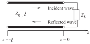
Figure \(\PageIndex{1}\): Transmission line of characteristic impedance \(Z_{0}\) and length \(\ell\) terminated in a load of impedance \(Z_{L}\).
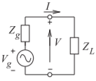
Figure \(\PageIndex{2}\): A Thevenin equivalent source with generator \(V_{g}\) and source impedance \(Z_{g}\) terminated in a load \(Z_{L}\).
\(\Gamma\) at the load is related to the impedance \(Z_{L}\) by
\[\label{eq:2}\Gamma(0)=\frac{Z_{L}-Z_{0}}{Z_{L}+Z_{0}} \]
where \(Z_{0}\) is the characteristic impedance of the connecting transmission line. This can also be written as
\[\label{eq:3}\Gamma(0)=\frac{Y_{0}-Y_{L}}{Y_{0}+Y_{L}} \]
where \(Y_{0} = 1/Z_{0}\) and \(Y_{L} = 1/Z_{L}\).
2.3.2 Reflection Coefficient with Complex Reference Impedance
Here the reflection coefficient of \(Z_{L}\) in Figure \(\PageIndex{2}\) will be developed with respect to the complex reference impedance \(Z_{g}\).The total voltage and current at the load are
\[\label{eq:4}V=V_{g}\frac{Z_{L}}{Z_{g}+Z_{L}} \]
and
\[\label{eq:5}I=\frac{V_{g}}{Z_{g}+Z_{L}} \]
To develop the reflection coefficient, first define equivalent forward- and backward-traveling waves. This can be done by imagining that between the generator and the load there is a transmission line of characteristic impedance \(Z_{g}\) which has infinitesimal length. The incident voltage and current waves \((V^{+}, I^{+})\) are the total voltage and current obtained when the generator is conjugately matched to the load (i.e., \(Z_{L} = Z_{g}^{\ast}\)). So the equations of forward-traveling voltage and current become\(^{2}\)
\[\label{eq:6}V^{+}=V_{g}\frac{Z_{g}^{\ast}}{Z_{g}+Z_{g}^{\ast}}=V_{g}Z_{g}^{\ast}2\mathcal{R}\{Z_{g}\} \]
\[\label{eq:7}I^{+}=V_{g}\frac{1}{2\mathcal{R}\{Z_{g}\}} \]
Now return to considering the actual load, \(Z_{L}\). The reflected voltage and current \((V^{−}, I^{−})\) are obtained by calculating the actual voltage and current at the source using the relationships
\[\label{eq:8}V=V^{+}+V^{-} \]
\[\label{eq:9}I=I^{+}+I^{-} \]
to determine the backward-traveling components. In Equations \(\eqref{eq:8}\) and \(\eqref{eq:9}\) the forward-traveling components are those in Equations \(\eqref{eq:6}\) and \(\eqref{eq:7}\). From Equation \(\eqref{eq:6}\),
\[\label{eq:10}V_{g}=V^{+}\frac{Z_{g}+Z_{g}^{\ast}}{Z_{g}^{\ast}} \]
and from Equations \(\eqref{eq:4}\), \(\eqref{eq:8}\), and \(\eqref{eq:10}\),
\[\begin{align}V^{-}&=V-V^{+}=V_{g}\frac{Z_{L}}{Z_{g}+Z_{L}}-V^{+}=\left[\frac{Z_{g}+Z_{g}^{\ast}}{Z_{g}^{\ast}}\frac{Z_{L}}{Z_{g}+Z_{L}}-1\right]V^{+}\nonumber \\ &=\left[\frac{Z_{g}Z_{L}+Z_{g}^{\ast}Z_{L}-Z_{g}^{\ast}Z_{g}-Z_{g}^{\ast}Z_{L}}{Z_{g}^{\ast}(Z_{g}+Z_{L})}\right]V^{+}\nonumber \\ \label{eq:11}&=\underbrace{\left(\frac{Z_{L}-Z_{g}^{\ast}}{Z_{L}+Z_{g}}\right)\frac{Z_{g}}{Z_{g}^{\ast}}}_{\Gamma^{V}}V^{+}=\Gamma^{V}V^{+}\end{align} \]
Similarly
\[\label{eq:12}I^{-}=\underbrace{-\left(\frac{Z_{L}-Z_{g}^{\ast}}{Z_{L}+Z_{g}}\right)\frac{Z_{g}}{Z_{g}^{\ast}}}_{\Gamma^{I}}I^{+}=\Gamma^{I}I^{+} \]
\(\Gamma^{V}\) is the voltage reflection coefficient, which is usually denoted as just \(\Gamma\), while \(\Gamma^{I}\) is the current reflection coefficient. It is clear that \(\Gamma^{V} =0=\Gamma^{I}\) when \(Z_{L} = Z_{g}^{\ast}\) and \(\Gamma^{V} = −\Gamma^{I} = (Z_{L} − R_{g})/(Z_{L} + R_{g})\) when \(Z_{g}\) is purely resistive (i.e., when \(Z_{g} = R_{g}\)). Generally the reflection coefficients are defined using a purely resistive \(Z_{g}\). This becomes the reference resistance, which is more commonly referred to as the reference impedance, \(Z_{0}\), or, if the same reference impedance is used throughout, the system impedance.
2.3.3 Two-Port \(S\) Parameters
Two-port \(S\) parameters are defined in terms of traveling waves on transmission lines with real characteristic impedance \(Z_{0}\) attached to each of the ports of the network, see Figure 2.1.1(b):
\[\label{eq:13}V_{1}^{-}=S_{11}V_{1}^{+}+S_{12}V_{2}^{+} \]
\[\label{eq:14}V_{2}^{-}=S_{21}V_{1}^{+}+S_{22}V_{2}^{+} \]
where \(S_{ij}\) are the individual \(S\) parameters. In matrix form the equations above become
\[\label{eq:15}\left[\begin{array}{c}{V_{1}^{-}}\\{V_{2}^{-}}\end{array}\right]=\left[\begin{array}{cc}{S_{11}}&{S_{12}} \\ {S_{21}}&{S_{22}}\end{array}\right]\left[\begin{array}{c}{V_{1}^{+}}\\{V_{2}^{+}}\end{array}\right]=\mathbf{S}\left[\begin{array}{c}{V_{1}^{+}}\\{V_{2}^{+}}\end{array}\right] \]
Individual \(S\) parameters are determined by measuring the forward- and backward-traveling waves with loads \(Z_{L} = Z_{0}\) at the ports. For the output line the load cannot reflect power and so \(V_{2}^{+}= 0\), then
\[\label{eq:16}S_{11}=\left.\frac{V_{1}^{-}}{V_{1}^{+}}\right|_{V_{2}^{+}=0} \]
The remaining three parameters are determined similarly and so \(S_{22}\) is found as
\[\label{eq:17}S_{22}=\left.\frac{V_{2}^{-}}{V_{2}^{+}}\right|_{V_{1}^{+}=0} \]
and the transmission parameter is
\[\label{eq:18}S_{21}=\left.\frac{V_{2}^{-}}{V_{1}^{+}}\right|_{V_{2}^{+}=0} \]
\(S_{21}\) is also called the transmission coefficient, \(T\). In the reverse direction,
\[\label{eq:19}S_{12}=\left.\frac{V_{1}^{-}}{V_{2}^{+}}\right|_{V_{1}^{+}=0} \]
In the above \(Z_{0}\) is referred to as the normalization impedance or equivalently the reference impedance. In some circumstances \(Z_{\text{REF}}\) is used to denote reference impedance to avoid possible confusion with a transmission line impedance that is not the same as the reference impedance. The \(S\) parameters here are also called normalized \(S\) parameters, and the \(S\) parameters are normalized to the same reference impedance at each port. Calling them normalized \(S\) parameters also carrys the additional meaning that the \(S\) parameters are referenced to the one real impedance.
The relationships between the two-port \(S\) parameters and the common network parameters are given in Table \(\PageIndex{1}\). It is interesting to note that \(S_{21}/S_{12} = z_{21}/z_{12} = y_{21}/y_{12} = h_{21}/h_{12}\). That is, the ratio of the forward to reverse parameters (at least for \(S,\: z,\: y,\) and \(h\) parameters) are the same and this ratio is one for a reciprocal device. An \(S\) parameter is a voltage ratio, so when it is expressed in decibels \(S_{ij}|_{\text{dB}} = 20 \log(S_{ij})\).
A reciprocal network has \(S_{12} = S_{21}\). If unit power flows into a two-port (with ports terminated in the reference impedance), a fraction, \(|S_{11}|^{2}\), is reflected and a further fraction, \(|S_{21}|^{2}\), is transmitted through the network.
Example \(\PageIndex{1}\): Two-Port \(S\) Parameters
What are the \(S\) parameters of a \(30\text{ dB}\) attenuator?
Solution
An attenuator is shown with a system impedance of \(Z_{0}\). An ideal attenuator has no reflection at each of the two ports when the attenuator is embedded in its system impedance. Thus \(\Gamma_{\text{in}} =0=\Gamma_{\text{out}}\). Since there is no reflection from the load or the source, this implies that \(S_{11} =0= S_{22}\).
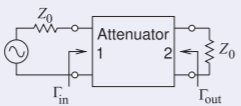
Figure \(\PageIndex{3}\)
Since this is a \(30\text{ dB}\) attenuator, the power delivered to the load impedance \(Z_{0}\) is \(30\text{ dB}\) below the power available from the source, thus \(S_{21} = −30\text{ dB} = 0.0316\). The attenuator is reciprocal and so \(S_{12} = S_{21}\). Thus the \(S\) parameters of the attenuator are
\[\label{eq:20}\mathbf{S}=\left[\begin{array}{cc}{0}&{0.0316} \\ {0.0316}&{0}\end{array}\right] \]
Note that the reference impedance did not need to be known to develop the \(S\) parameters.
| \(S\) | In terms of \(S\) | |
|---|---|---|
| \(z\) | \(Z_{11}'=z_{11}Z_{0}\quad Z_{12}'=z_{12}Z_{0}\) | \(Z_{21}'=z_{21}Z_{0}\quad Z_{22}'=z_{22}Z_{0}\) |
| \(\begin{aligned} \delta_{z}&= (1+z_{11})(1+z_{22})-z_{12}z_{21} \\ S_{11}&=[(z_{11}-1)(z_{22}+1)-z_{12}z_{21}]/\delta_{z} \\ S_{12}&=2z_{12}/\delta_{z} \\ S_{21}&=2z_{21}/\delta_{z} \\ S_{22}&=[(z_{11}+1)(z_{22}-1)-z_{12}z_{21}]/\delta_{z}\end{aligned}\) | \(\begin{aligned}\delta_{S}&=(1-S_{11})(1-S_{22})-S_{12}S_{21} \\ z_{11}&=[(1+S_{11})(1-S_{22})+S_{12}S_{21}]/\delta_{S} \\ z_{12}&=2S_{12}/\delta_{S} \\ z_{21}&=2S_{21}/\delta_{S} \\ z_{22}&=[(1-S_{11})(1+S_{22})+S_{12}S_{21}]/\delta_{S}\end{aligned}\) | |
| \(y\) | \(Y_{11}'=y_{11}/Z_{0}\quad Y_{12}'=y_{12}/Z_{0}\) | \(Y_{21}'=y_{21}/Z_{0}\quad Y_{22}'=y_{22}/Z_{0}\) |
| \(\begin{aligned}\delta_{y}&=(1+y_{11})(1+y_{22})-y_{12}y_{21} \\ S_{11}&=[(1-y_{11})(1+y_{22})+y_{12}y_{21}]/\delta_{y} \\ S_{12}&=-2y_{12}/\delta_{y} \\ S_{21}&=-2y_{21}/\delta_{y} \\ S_{22} &=[(1+y_{11})(1-y_{22})+y_{12}y_{21}]/\delta_{y}\end{aligned}\) | \(\begin{aligned}\delta_{S}&=(1+S_{11})(1+S_{22})-S_{12}S_{21}\\ y_{11}&=[(1-S_{11})(1+S_{22})+S_{12}S_{21}]/\delta_{S} \\ y_{12}&=-2S_{12}/\delta_{S} \\ y_{21}&=-2S_{21}/\delta_{S} \\ y_{22}&=[(1+S_{11})(1-S_{22})+S_{12}S_{21}]/\delta_{S}\end{aligned}\) | |
| \(h\) | \(H_{11}'=h_{11}Z_{0}\quad H_{12}'=h_{12}\) | \(H_{21}'=h_{21}\quad H_{22}'=h_{22}/Z_{0}\) |
| \(\begin{aligned}\delta_{h}&=(1+h_{11})(1+h_{22})-h_{12}h_{21} \\ S_{11}&=[(h_{11}-1)(h_{22}+1)-h_{12}h_{21}]/\delta_{h} \\ S_{12}&=2h_{12}/\delta_{h} \\ S_{21}&=-2h_{21}/\delta_{h} \\ S_{22}&=[(1+h_{11})(1-h_{22})+h_{12}h_{21}]/\delta_{h}\end{aligned}\) | \(\begin{aligned}\delta_{S}&=(1-S_{11})(1+S_{22})+S_{12}S_{21} \\ h_{11}&=[(1+S_{11})(1+S_{22})-S_{12}S_{21}]/\delta_{S} \\ h_{12}&=2S_{12}/\delta_{S} \\ h_{21}&=-2S_{21}/\delta_{S} \\ h_{22}&=[(1-S_{11})(1-S_{22})-S_{12}S_{21}]/\delta_{S}\end{aligned}\) |
Table \(\PageIndex{1}\): Two-port \(S\) parameter conversion chart. The \(z,\: y,\) and \(h\) parameters are normalized to \(Z_{0}\). \(Z′,\: Y′,\) and \(H′\) are the actual parameters. For \(ABCD\) parameter conversion see Section 2.7.2.
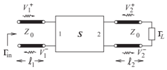
Figure \(\PageIndex{4}\): A terminated two-port network with transmission lines of infinitesimal length at the ports.
2.3.4 Input Reflection Coefficient of a Terminated Two-Port Network
A two-port is shown in Figure \(\PageIndex{4}\) that is terminated at Port \(\mathsf{2}\) in a load with a reflection coefficient \(\Gamma_{L}\). The lines at each of the ports are of infinitesimal length (i.e., \(\ell_{1} → 0\) and \(\ell_{2} → 0\)) and are used to make it easier to visualize the separation of the voltage into forward- and backward-traveling components. The aim in this section is to develop a formula for the input reflection coefficient \(\Gamma_{\text{in}} = V_{1}^{−}/V_{1}^{+}\). For the circuit in Figure \(\PageIndex{4}\) three equations can be developed:
\[\begin{align}\label{eq:21}V_{1}^{-}&=S_{11}V_{1}^{+}+S_{12}V_{2}^{+} \\ \label{eq:22}V_{2}^{-}&=S_{21}V_{1}^{+}+S_{22}V_{2}^{+} \\ \label{eq:23}V_{2}^{+}&=\Gamma_{L}V_{2}^{-},\quad\text{i.e.,}\quad V_{2}^{-}=V_{2}^{+}/\Gamma_{L}\end{align} \]
Note that \(V_{2}^{−}\) is the voltage wave that leaves the two-port but is incident on the load \(\Gamma_{L}\). The aim here is to eliminate \(V_{2}^{+}\) and \(V_{2}^{−}\). Substituting Equation
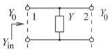
Figure \(\PageIndex{5}\): Shunt element in the form of a two-port.
\(\eqref{eq:23}\) into Equation \(\eqref{eq:22}\) leads to
\[\begin{align}\label{eq:24}V_{2}^{+}/\Gamma_{L}&=S_{21}V_{1}^{+}+S_{22}V_{2}^{+} \\ \label{eq:25}V_{2}^{+}\left(\frac{1-S_{22}\Gamma_{L}}{\Gamma_{L}}\right)&=S_{21}V_{1}^{+} \\ \label{eq:26}V_{2}^{+}&=\left(\frac{S_{21}\Gamma_{L}}{1-S_{22}\Gamma_{L}}\right)V_{1}^{+}\end{align} \]
Now substituting Equation \(\eqref{eq:26}\) in Equation \(\eqref{eq:21}\) yields
\[\label{eq:27}V_{1}^{-}=S_{11}V_{1}^{+}+S_{12}\left(\frac{S_{21}\Gamma_{L}}{1-S_{22}\Gamma_{L}}\right)V_{1}^{+} \]
and so
\[\label{eq:28}\Gamma_{\text{in}}=S_{11}+\frac{S_{12}S_{21}\Gamma_{L}}{1-S_{22}\Gamma_{L}} \]
2.3.5 Evaluation of the Scattering Parameters of an Element
Scattering parameters can be derived analytically for various circuit configurations and in this section the procedure is illustrated for the shunt element of Figure \(\PageIndex{5}\). The procedure to find \(S_{11}\) is to match Port \(\mathsf{2}\) so that \(V_{2}^{+}= 0\), then \(S_{11}\) is the reflection coefficient at Port \(\mathsf{1}\):
\[\label{eq:29}S_{11}=\frac{Y_{0}-Y_{\text{in}}}{Y_{0}+Y_{\text{in}}} \]
where \(Y_{\text{in}} = Y_{0} + Y\), since the matched termination at Port \(\mathsf{2}\) (i.e., \(Y_{0} = 1/Z_{0}\)) shunts the admittance \(Y\). Thus
\[\label{eq:30}S_{11}=\frac{Y_{0}-Y_{0}-Y}{2Y_{0}+Y}=\frac{-Y}{2Y_{0}+Y} \]
From the symmetry of the two-port,
\[\label{eq:31}S_{22}=S_{11} \]
\(S_{21}\) is evaluated by determining the transmitted wave, \(V_{2}^{−}\), with the output line matched so that again an admittance, \(Y_{0}\), is placed at Port \(\mathsf{2}\) and \(V_{2}^{+} = 0\). After some algebraic manipulation,
\[\label{eq:32}S_{21}=2Y_{0}/(Y+2Y_{0}) \]
is obtained. Since this is clearly a reciprocal network, \(S_{12} = S_{21}\) and all four \(S\) parameters are obtained. A similar procedure of selectively applying matched loads is used to obtain the \(S\) parameters of other networks.
Example \(\PageIndex{2}\): Calculation of the \(S\) Parameters of a Two-Port Network
Derive the two-port \(50\:\Omega\text{ S}\) parameters of the resistive circuit to the right.
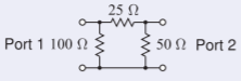
Figure \(\PageIndex{6}\)
Solution
\(\underline{\text{Calculation of }S_{11}.}\) This involves terminating Port \(\mathsf{2}\) in the system reference impedance, \(50\:\Omega\), and then calculating the input impedance of the augmented network. This is then converted to a reflection coefficient, which here is \(S_{11}\). The circuit for calculation is to the right. Now
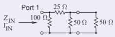
Figure \(\PageIndex{7}\)
\[\label{eq:33}Z_{\text{IN}}=100\parallel [25\:$\:(50\parallel 50)]\:\Omega=100\parallel 50\:\Omega=33.33\:\Omega \]
where \(\parallel\) indicates the parallel-connection calculation and \($\) indicates the series-connection calculation. Thus
\[\label{eq:34}S_{11}=\Gamma_{\text{IN}}=\frac{Z_{\text{IN}}-Z_{0}}{Z_{\text{IN}}+Z_{0}}=\frac{33.33-50}{33.33+50}=-0.2 \]
\(\underline{\text{Calculation of }S_{21}.}\) This involves terminating Port \(\mathsf{2}\) in the system reference impedance, \(50\:\Omega\), and then calculating the forward-traveling voltage wave at Port \(\mathsf{1}\) and the reverse-traveling voltage wave at Port \(\mathsf{2}\). Note that the reverse-traveling voltage wave at Port \(\mathsf{2}\) is leaving the two-port.
Since there is no wave reflected from the termination at Port \(\mathsf{2}\), the total voltage at Port \(\mathsf{2}\) is just \(V_{2}^{−}\). The circuit for calculation is on the right.
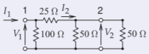
Figure \(\PageIndex{8}\)
\[\label{eq:35}V_{1}=V_{1}^{+}+V_{1}^{-}=V_{1}^{+}(1+S_{11})\to V_{1}^{+}=\frac{V_{1}}{1+S_{11}}=1.25V_{1} \]
The voltage at Port \(\mathsf{1}\) is
\[\label{eq:36}V_{1}=I_{1}Z_{\text{IN}}=33.33I_{1}\to V_{1}^{+}=1.25\cdot 33.33I_{1}=41.66I_{1} \]
The next step is to find an expression for \(I_{2}\):
\[\label{eq:37}V_{1}=I_{1}Z_{\text{IN}}=33.33I_{1}=I_{2}(25\:$\:50\parallel 50)=50I_{2} \]
Rearranging,
\[\label{eq:38}I_{2}=I_{1}\frac{33.33}{50}=0.6667I_{1} \]
Now
\[\label{eq:39}V_{2}^{-}=V_{2}=I_{2}(50\parallel 50)=25I_{2}=16.67I_{1} \]
So
\[\label{eq:40}S_{21}=\frac{V_{2}^{-}}{V_{1}^{+}}=\frac{16.67}{41.66}=0.4 \]
\(\underline{\text{Calculation of }S_{12}.}\) The two-port is a reciprocal network (as are all networks with only lumped \(R,\: L,\) and \(C\) elements) and so \(S_{12} = S_{21}\).
\(\underline{\text{Calculation of }S_{22}.}\) Using a similar procedure to that used for finding \(S_{11}\), the circuit for the calculation is on the right:
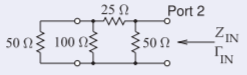
Figure \(\PageIndex{9}\)
\[\label{eq:41}Z_{\text{IN}}=50\parallel [25\:$\:(100\parallel 50)]\:\Omega=50\parallel (25\:$\:33.33)=50\parallel 58.33=26.92\:\Omega \]
Therefore
\[\label{eq:42}S_{22}=\Gamma_{\text{IN}}=\frac{26.92-50}{26.92+50}=-0.3 \]
Collecting the individual \(S\) parameters:
\[\label{eq:43}\mathbf{S}=\left[\begin{array}{cc}{-0.2}&{0.4}\\{0.4}&{-0.3}\end{array}\right] \]
2.3.6 Properties of a Two-Port in Terms of \(S\) Parameters
The properties of most interest are whether the two-port network is lossless, passive, or reciprocal.
If a network is lossless, all of the power input to the network must leave the network. The power incident on Port \(\mathsf{1}\) of a network is
\[\label{eq:44}P_{1}^{+}=\left|\frac{\frac{1}{2}V_{1}^{+}}{Z_{0}}\right|^{2} \]
and the power leaving Port \(\mathsf{1}\) is
\[\label{eq:45}P_{1}^{-}=\left|\frac{\frac{1}{2}V_{1}^{-}}{Z_{0}}\right|^{2} \]
This can be repeated for Port \(\mathsf{2}\) and the factor \(\frac{1}{2}/Z_{0}\) appears in all expressions.
So cancelling this factor, the condition for the network to be lossless is
\[\label{eq:46}|S_{11}|^{2}+|S_{21}|^{2}=1\quad\text{and}\quad |S_{12}|^{2}+|S_{22}|^{2}=1 \]
For a network to be passive, no more power can leave the network than enters it. So the condition for passivity is
\[\label{eq:47}|S_{11}|^{2}+|S_{21}|^{2}\leq 1\quad\text{and}\quad |S_{12}|^{2}+|S_{22}|^{2}\leq 1 \]
Reciprocity requires that \(S_{21} = S_{12}\).
2.3.7 Scattering Transfer or \(T\) Parameters
\(S\) parameters relate reflected waves to incident waves, thus mixing the quantities at the input and output ports. However, in dealing with cascaded networks it is preferable to relate the traveling waves at the input ports to the output ports. Such parameters are called the scattering transfer (or \(^{S}T\)) parameters, which for a two-port network are defined by
\[\label{eq:48}\left[\begin{array}{c}{V_{1}^{-}}\\{V_{1}^{+}}\end{array}\right]=\left[\begin{array}{cc}{^{S}T_{11}}&{^{S}T_{12}}\\{^{S}T_{21}}&{^{S}T_{22}}\end{array}\right]\left[\begin{array}{c}{V_{2}^{+}}\\{V_{2}^{-}}\end{array}\right] \]
where
\[\label{eq:49}^{S}\mathbf{T}=\left[\begin{array}{cc}{^{S}T_{11}}&{^{S}T_{12}}\\{^{S}T_{21}}&{^{S}T_{22}}\end{array}\right] \]
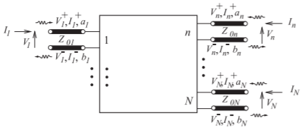
Figure \(\PageIndex{10}\): \(N\)-port network with traveling voltage and current waves.
The two-port \(^{S}T\) parameters and \(S\) parameters are related by
\[\label{eq:50}\left[\begin{array}{cc}{^{S}T_{11}}&{^{S}T_{12}}\\{^{S}T_{21}}&{^{S}T_{22}}\end{array}\right]=\left[\begin{array}{cc}{-(S_{11}S_{22}-S_{12}S_{21})/S_{21}}&{(S_{11}/S_{21})} \\ {-(S_{22}/S_{21})}&{(1/S_{21})}\end{array}\right] \]
and
\[\label{eq:51}\left[\begin{array}{cc}{S_{11}}&{S_{12}}\\{S_{21}}&{S_{22}}\end{array}\right]=\left[\begin{array}{cc}{^{S}T_{12}\:^{S}T_{22}^{-1}}&{(^{S}T_{11}-^{S}T_{12}\:^{S}T_{22}^{-1}\:^{S}T_{21})}\\{^{S}T_{22}^{-1}}&{-^{S}T_{22}^{-1}\:^{S}T_{21}}\end{array}\right] \]
Very often the \(^{S}T\) parameters are called \(T\) parameters, but there are at least two types of \(T\) parameters, so it is necessary to be specific. (Another form will be introduced in Section 2.6.) If networks A and B have parameters \(^{S}\mathbf{T}_{A}\) and \(^{S}\mathbf{T}_{B}\), then the \(^{S}\mathbf{T}\) parameters of the cascaded network are
\[\label{eq:52}^{S}\mathbf{T}=^{S}\mathbf{T}_{A}\cdot ^{S}\mathbf{T}_{B} \]
There are two forms of the scattering \(T\) parameters. Here the scattering transfer parameters are designated as the \(^{S}T\) parameters but often \(T\) on its own is used. The other more common form are the chain scattering parameters which will be considered in Section 2.6.