2.6: \(T\) or Chain Scattering Parameters of Cascaded Two-Port Networks

The \(T\) parameters, also known as chain scattering parameters, are a cascadable form of scattering parameters. They are similar to regular \(S\) parameters and can be expressed in terms of the \(a\) and \(b\) root power waves or traveling voltage waves. Two two-port networks, A and B, in cascade are shown in Figure \(\PageIndex{1}\). Here \((A)\) and \((B)\) are used as superscripts to distinguish the parameters of each two-port network, but the subscripts \(A\) and \(B\) are used for matrix quantities. Since

\[\label{eq:1}a_{2}^{(A)}=b_{1}^{(B)}\quad\text{and}\quad b_{2}^{(A)}=a_{1}^{(B)} \]

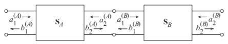
Figure \(\PageIndex{1}\): Two cascaded two-ports.

it is convenient to put the \(a\) and \(b\) parameters in cascadable form, leading to the following two-port chain matrix or \(T\) matrix representation (with respect to Figure 2.4.3):

\[\label{eq:2} \left[\begin{array}{c}{a_{1}}\\{b_{1}}\end{array}\right] =\left[\begin{array}{cc}{T_{11}}&{T_{12}}\\{T_{21}}&{T_{22}}\end{array}\right]\left[\begin{array}{c}{b_{2}}\\{a_{2}}\end{array}\right] \]

where the \(\text{T}\) matrix or chain scattering matrix is

\[\label{eq:3}\mathbf{T}=\left[\begin{array}{cc}{T_{11}}&{T_{12}}\\{T_{21}}&{T_{22}}\end{array}\right] \]

\(\mathbf{T}\) is very similar to the scattering transfer matrix \((\:^{S}\mathbf{T})\) of Section 2.3.7. The only difference is the ordering of the \(a\) and \(b\) components. You will come across both forms, so be careful that you understand which is being used. Both forms are used for the same function—cascading two-port networks. The relationships between \(\mathbf{T}\) and \(\mathbf{S}\) are given by

\[\label{eq:4}\mathbf{T}=\left[\begin{array}{cc}{S_{21}^{-1}}&{-S_{21}^{-1}S_{22}}\\{S_{21}^{-1}S_{11}}&{S_{12}-S_{11}S_{21}^{-1}S_{22}}\end{array}\right] \]

\[\label{eq:5}\mathbf{S}=\left[\begin{array}{cc}{T_{21}T_{11}^{-1}}&{T_{22}-T_{21}T_{11}^{-1}T_{12}}\\{T_{11}^{-1}}&{-T_{11}^{-1}T_{12}}\end{array}\right] \]

For a two-port network, using Equations \(\eqref{eq:1}\) and \(\eqref{eq:2}\),

\[\label{eq:6}\left[\begin{array}{c}{a_{1}^{(A)}}\\{b_{1}^{(A)}}\end{array}\right]=\mathbf{T}_{A}\left[\begin{array}{c}{b_{2}^{(A)}}\\{a_{2}^{(A)}}\end{array}\right]\quad\text{and}\quad\left[\begin{array}{c}{a_{1}^{(B)}}\\{b_{1}^{(B)}}\end{array}\right]=\mathbf{T}_{B}\left[\begin{array}{c}{b_{2}^{(B)}}\\{a_{2}^{(B)}}\end{array}\right] \]

thus

\[\label{eq:7}\left[\begin{array}{c}{a_{1}^{(A)}}\\{b_{1}^{(A)}}\end{array}\right]=\mathbf{T}_{A}\mathbf{T}_{B}\left[\begin{array}{c}{b_{2}^{(B)}}\\{a_{2}^{(B)}}\end{array}\right] \]

For \(n\) cascaded two-port networks, Equation \(\eqref{eq:7}\) generalizes to

\[\label{eq:8}\left[\begin{array}{c}{a_{1}^{(1)}}\\{b_{1}^{(1)}}\end{array}\right]=\mathbf{T}_{1}\mathbf{T}_{2}\ldots\mathbf{T}_{n}\left[\begin{array}{c}{b_{2}^{(n)}}\\{a_{2}^{(n)}}\end{array}\right] \]

and so the \(\mathbf{T}\) matrix of the cascaded network is the matrix product of the \(\mathbf{T}\) matrices of the individual two-ports.

Previously, in Section 2.3.7, the scattering transfer parameters were introduced. Both the chain scattering parameters and scattering transfer parameters are referred to as \(T\) parameters. Be careful to denote which form is being used.

Example \(\PageIndex{1}\): Development of Chain Scattering Parameters

Derive the \(T\) parameters of the two-port network to the right using a reference impedance \(Z_{0}\).

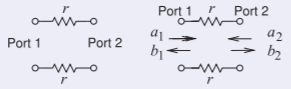
Figure \(\PageIndex{2}\)

Solution

\(\underline{\text{Derivation of }T_{11}}\)

Terminate Port \(\mathsf{2}\) in a matched load so that \(a_{2} = 0\). Then Equation \(\eqref{eq:2}\) becomes \(a_{1} = T_{11}b_{2}\) and \(b_{1} = T_{21}b_{2}\) so

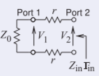
Figure \(\PageIndex{3}\)

\[\label{eq:9}\Gamma_{\text{in}}=b_{1}/a_{1}=T_{21}/T_{11} \]

Now \(Z_{\text{in}}=2r+Z_{0}\), therefore

\[\begin{aligned}\Gamma_{\text{in}}&=\frac{Z_{\text{in}}-Z_{0}}{Z_{\text{in}}+Z_{0}} \\ &=\frac{2r+Z_{0}-Z_{0}}{2r+Z_{0}+Z_{0}}=\frac{r}{r+Z_{0}}\end{aligned}\nonumber \]

Thus

\[\label{eq:10}\Gamma_{\text{in}}=\frac{T_{21}}{T_{11}}=\frac{r}{r+Z_{0}} \]

The next stage is relating \(b_{2}\) to \(a_{1}\) and since both ports have the same reference impedance \(a\) and \(b\) can be replaced by traveling voltages

\[\begin{aligned}V_{1}=(V_{1}^{+}+V_{1}^{-})&=V_{1}^{+}(1+\Gamma_{\text{in}}) \\ &=V_{1}^{+}\frac{2r+Z_{0}}{r+Z_{0}}\end{aligned}\nonumber \]

Using voltage division (and since \(V_{2}^{+} = a_{2} = 0\))

\[\begin{align}V_{2}=V_{2}^{-}&=\frac{Z_{0}}{2r+Z_{0}}V_{1}\nonumber \\ &=V_{1}^{+}\frac{Z_{0}}{2r+Z_{0}}\frac{2r+Z_{0}}{r+Z_{0}}\nonumber \\ V_{2}^{-}&=V_{1}^{+}\frac{Z_{0}}{r+Z_{0}}\nonumber \\ \label{eq:11}T_{11}&=\frac{V_{1}^{+}}{V_{2}^{-}}=\frac{a_{1}}{b_{2}}=\frac{r+Z_{0}}{Z_{0}}\end{align} \]

\(\underline{\text{Derivation of }T_{21}}\)

Combining Equations \(\eqref{eq:10}\) and \(\eqref{eq:11}\)

\[\label{eq:12}T_{21}=\Gamma_{\text{in}}T_{11}=\frac{r}{r+Z_{0}}\frac{r+Z_{0}}{Z_{0}}=\frac{r}{Z_{0}} \]

\(\underline{\text{Derivation of }T_{22}}\)

Terminate Port \(\mathsf{2}\) in a matched load so that \(a_{1} = 0\). Then Equation \(\eqref{eq:2}\) becomes

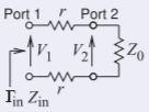
Figure \(\PageIndex{4}\)

\[\begin{align}0&=T_{11}b_{2}+T_{12}a_{2}\nonumber \\ \label{eq:13}\Gamma_{\text{in}}&=\frac{b_{2}}{a_{2}}=\frac{-T_{12}}{T_{11}}\to T_{12}=-T_{11}\Gamma_{\text{in}} \\ b_{1}&=T_{21}b_{2}+T_{22}a_{2} \\ \label{eq:14}\frac{b_{1}}{a_{2}}&=T_{21}\frac{b_{2}}{a_{2}}+T_{22}\end{align} \]

Now \(Z_{\text{in}} = 2r + Z_{0}\) and so

\[\label{eq:15}\Gamma_{\text{in}}=\frac{2r+Z_{0}-Z_{0}}{2r+Z_{0}+Z_{0}}=\frac{r}{r+Z_{0}} \]

Using voltage division

\[\begin{align}V_{1}&=V_{1}^{-}=\frac{Z_{0}}{2r+Z_{0}}V_{2}=\frac{Z_{0}}{2r+Z_{0}}V_{2}^{+}(1+\Gamma_{\text{in}})\nonumber \\ &=V_{2}^{+}\frac{Z_{0}}{2r+Z_{0}}\frac{2r+Z_{0}}{r+Z_{0}}=V_{2}^{+}\frac{Z_{0}}{r+Z_{0}}\nonumber \\ \label{eq:16}\frac{V_{1}^{-}}{V_{2}^{+}}&=\frac{b_{1}}{a_{2}}=\frac{Z_{0}}{r+Z_{0}}\end{align} \]

Substituting Equations \(\eqref{eq:15}\) and \(\eqref{eq:16}\) in Equation \(\eqref{eq:14}\) and rearranging

\[T_{22}=\frac{Z_{0}}{r+Z_{0}}-T_{21}\frac{r}{r+Z_{0}}\nonumber \]

Combining this with Equation \(\eqref{eq:12}\)

\[\label{eq:17}T_{22}=\frac{Z_{0}}{r+Z_{0}}-\frac{r}{Z_{0}}\frac{r}{r+Z_{0}}=\frac{Z_{0}^{2}-r^{2}}{Z_{0}(r+Z_{0})} \]

\(\underline{\text{Derivation of }T_{12}}\)

Combining Equations \(\eqref{eq:11}\), \(\eqref{eq:13}\) and \(\eqref{eq:15}\)

\[\label{eq:18}T_{12}=-\frac{r+Z_{0}}{Z_{0}}\frac{r}{r+Z_{0}}=-\frac{r}{Z_{0}} \]

\(\underline{\text{Summary}}\):

The chain scattering matrix \((T)\) parameters are given in Equations \(\eqref{eq:11}\), \(\eqref{eq:12}\), \(\eqref{eq:17}\), and \(\eqref{eq:18}\).

Example \(\PageIndex{2}\): Cascading Chain Scattering Parameters

Develop the chain scattering parameters of the network to the right. Use a reference impedance \(Z_{\text{REF}} = Z_{0}\), the characteristic impedance of the lines.

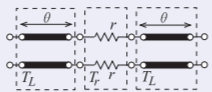
Figure \(\PageIndex{5}\)

Solution

The network comprises a transmission line of electrical length \(\theta\) in cascade with a resistive network and another line of the same electrical length. From Equation (2.5.3) the scattering parameters of the transmission line are

\[\label{eq:19}\mathbf{S}_{L}=\left[\begin{array}{cc}{0}&{\text{e}^{-\jmath\theta}}\\{\text{e}^{-\jmath\theta}}&{0}\end{array}\right] \]

From Equation \(\eqref{eq:4}\) the chain scattering matrix of the line is

\[\label{eq:20}\mathbf{T}_{L}=\left[\begin{array}{cc}{\text{e}^{\jmath\theta}}&{0}\\{0}&{\text{e}^{-\jmath\theta}}\end{array}\right] \]

From Example \(\PageIndex{1}\) the chain scattering matrix of the resistive network is

\[\label{eq:21}\mathbf{T}_{r}=\frac{1}{Z_{0}}\left[\begin{array}{cc}{gr+Z_{0}}&{-r}\\{r}&{(Z_{0}^{2}-r^{2})/(r+Z_{0})}\end{array}\right] \]

Yielding the chain scattering matrix of the cascade;

\[\label{eq:22}\begin{array}{l}{T_{LrL}=T_{L}T_{r}T_{L}} \\ {\frac{1}{Z_{0}}\left[\begin{array}{cc}{(r+Z_{0})\text{e}^{2\jmath\theta}}&{-r}\\{r}&{(Z_{0}^{2}-r^{2})/(r+Z_{0})\text{e}^{-2\jmath\theta}}\end{array}\right]}\end{array} \]

Example \(\PageIndex{3}\): Input Reflection Coefficient of a Terminated Two-Port

What is the input reflection coefficient in terms of chain scattering parameters of the terminated two-port to the right where the two-port is described by its chain scattering parameters.

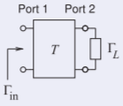
Figure \(\PageIndex{6}\)

Solution

The chain scattering parameter relations are

\[\left[\begin{array}{c}{a_{1}}\\{b_{1}}\end{array}\right]=\left[\begin{array}{cc}{T_{11}}&{T_{12}}\\{T_{21}}&{T_{22}}\end{array}\right]\left[\begin{array}{c}{b_{2}}\\{a_{22}}\end{array}\right]\nonumber \]

Expanding this matrix equation and using the substitution \(a_{2} = \Gamma_{L}b_{2}\)

\[\begin{align}\label{eq:23}a_{1}&=T_{11}b_{2}+T_{12}\Gamma_{L}b_{2} \\ \label{eq:24}b_{1}&+T_{21}b_{2}+T_{22}\Gamma_{L}b_{2}\end{align} \]

Multiplying Equation \(\eqref{eq:23}\) by \((T_{21} + T_{22}\Gamma_{L})\) and Equation \(\eqref{eq:24}\) by \((T_{11} +T_{12}\Gamma_{L})\) and then subtracting

\[\begin{aligned}(T_{21} + T_{22}\Gamma_{L})a_{1} &= (T_{21} + T_{22}\Gamma_{L})(T_{11}b_{2} + T_{12}\Gamma_{L})b_{2}\nonumber \\ (T_{11} + T_{12}\Gamma_{L})b_{1} &= (T_{11} + T_{12}\Gamma_{L})(T_{21}b_{2} + T_{22}\Gamma_{L})b_{2}\nonumber \\ (T_{21} + T_{22}\Gamma_{L})a_{1} &= (T_{11} + T_{12}\Gamma_{L})b_{1}\nonumber\end{aligned} \nonumber \]

Thus the input reflection coefficient is

\[\label{eq:25}\Gamma_{\text{in}}=\frac{b_{1}}{a_{1}}=\frac{T_{21}+T_{22}\gamma_{L}}{T_{11}+T_{12}\gamma_{L}} \]

Now consider a transmission line of electrical length \(\theta\) and characteristic impedance \(Z_{0}\) (see the figure b) in cascade with the two-port.

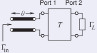
Figure \(\PageIndex{7}\)

The input reflection coefficient now is found by first determining the total chain scattering matrix of the cascade:

\[\begin{aligned}^{\mathbf{T}}\mathbf{T}&=\mathbf{T}_{\mathbf{L}}\mathbf{T}=\left[\begin{array}{cc}{\text{e}^{\jmath\theta}}&{0}\\{0}&{\text{e}^{-\jmath\theta}}\end{array}\right]\left[\begin{array}{cc}{T_{11}}&{T_{12}}\\{T_{21}}&{T_{22}}\end{array}\right]\nonumber \\ &=\left[\begin{array}{cc}{T_{11}\text{e}^{\jmath\theta}}&{T_{12}\text{e}^{\jmath\theta}}\\{T_{21}\text{e}^{-\jmath\theta}}&{T_{22}\text{e}^{-\jmath\theta}}\end{array}\right]\left[\begin{array}{cc}{^{T}T_{11}}&{^{T}T_{12}}\\{^{T}T_{21}}&{^{T}T_{22}}\end{array}\right]\nonumber\end{aligned} \nonumber \]

Thus the input reflection coefficient is now

\[\begin{align}\Gamma_{\text{in}}&=\frac{b_{1}}{a_{1}}=\frac{^{T}T_{21}+\:^{T}T_{22}\Gamma_{L}}{^{T}T_{11}+\:^{T}T_{12}\Gamma_{L}}\nonumber \\ &=\frac{T_{21}\text{e}^{-\jmath\theta}+T_{22}\text{e}^{-\jmath\theta}\Gamma_{L}}{T_{11}\text{e}^{\jmath\theta}+T_{12}\text{e}^{\jmath\theta}\Gamma_{L}}\nonumber \\ \label{eq:26}&=\text{e}^{-2\jmath\theta}\left(\frac{T_{21}+T_{22}\Gamma_{L}}{T_{11}+T_{12}\Gamma_{L}}\right)\end{align} \]

If the load is now a short circuit \(\Gamma_{L} = −1\) and the input reflection coefficient of the line and two-port cascade is

\[\label{eq:27}\Gamma_{\text{in}}=\text{e}^{-2\jmath\theta}\left(\frac{T_{21}-T_{22}}{T_{11}-T_{12}}\right) \]

2.6.1 Terminated Two-Port Network

A two-port with Port 2 terminated in a load with reflection coefficient \(\Gamma_{L}\) is shown in Figure 2.7.1 and \(a_{2} =\Gamma_{L}b_{2}\). Substituting this in Equation \(\eqref{eq:2}\) leads to

\[a_{1} = (T_{11} + T_{12}\Gamma_{L})b_{2}\quad\text{and}\quad b_{1} = (T_{21} + T_{22}\Gamma_{L})b_{2}\nonumber \]

eliminating \(b_{2}\) results in

\[\label{eq:28}\Gamma_{\text{in}}=\frac{b_{1}}{a_{1}}=\frac{T_{21}+T_{22}\Gamma_{L}}{T_{11}+T_{12}\Gamma_{L}} \]