2.7: Scattering Parameter Two-Port Relationships

2.7.1 Change in Reference Plane

It is often necessary during \(S\) parameter measurements of two-port devices to measure components at a position different from that actually desired. An example is shown in Figure \(\PageIndex{2}\)(a). From direct measurement the \(S\) parameters are obtained, and thus the \(\mathbf{T}\) matrix at Planes \(\mathsf{1}\) and \(\mathsf{2}\). However, \(\mathbf{T}_{\text{DUT}}\) referenced to Planes \(\mathsf{1}'\) and \(\mathsf{2}'\) is required. Now,

\[\label{eq:1}\mathbf{T}=\mathbf{T}_{\theta_{1}}\mathbf{T}_{\text{DUT}}\mathbf{T}_{\theta_{2}} \]

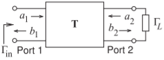
Figure \(\PageIndex{1}\): Terminated two-port network.

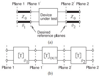
Figure \(\PageIndex{2}\): Two-port measurement setup: (a) a two-port comprising a device under test (\(\text{DUT}\)) and transmission line sections that create a reference plane at Planes \(\mathsf{1}\) and \(\mathsf{2}\); and (b) representation as cascaded two-port networks.

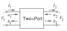
Figure \(\PageIndex{3}\): Two-port with parameters suitable for defining \(S\) and \(ABCD\) parameters.

and so

\[\label{eq:2}\mathbf{T}_{\text{DUT}}=\mathbf{T}_{\theta_{1}}^{-}\mathbf{TT}_{\theta_{2}}^{-1} \]

A section of line with electrical length \(\theta\) and port impedances equal to its characteristic impedance has

\[\label{eq:3}\mathbf{S}=\left[\begin{array}{cc}{0}&{\text{e}^{-\jmath\theta}}\\{\text{e}^{-\jmath\theta}}&{0}\end{array}\right] \]

and

\[\label{eq:4}\mathbf{T}_{\theta}=\left[\begin{array}{cc}{\text{e}^{\jmath\theta}}&{0}\\{0}&{\text{e}^{-\jmath\theta}}\end{array}\right] \]

Therefore Equation \(\eqref{eq:2}\) becomes

\[\label{eq:5}\mathbf{T}_{\text{DUT}}=\left[\begin{array}{cc}{T_{11}\text{e}^{-\jmath(\theta_{1}+\theta_{2})}}&{T_{12}\text{e}^{-\jmath(\theta_{1}-\theta_{2})}} \\ {T_{21}\text{e}^{\jmath(\theta_{1}-\theta_{2})}}&{T_{22}\text{e}^{\jmath(\theta_{1}+\theta_{2})}}\end{array}\right] \]

and then the desired \(S\) parameters of the \(\text{DUT}\) are obtained as

\[\label{eq:6}\mathbf{S}_{\text{DUT}}=\left[\begin{array}{cc}{S_{11}\text{e}^{\jmath 2\theta_{1}}}&{S_{12}\text{e}^{\jmath(\theta_{1}+\theta_{2})}}\\{S_{21}\text{e}^{\jmath(\theta_{1}+\theta_{2})}}&{S_{22}\text{e}^{\jmath 2\theta_{2}}}\end{array}\right] \]

2.7.2 Conversion Between \(S\) and \(ABCD\) Parameters

Figure \(\PageIndex{3}\) can be used to relate the parameters of the two views of the network. If both ports have the same reference impedance \(Z_{0}\), then

\[\left[\begin{array}{c}{V_{1}}\\{I_{1}}\end{array}\right]=\left[\begin{array}{cc}{A}&{B}\\{C}&{D}\end{array}\right]\left[\begin{array}{c}{V_{2}}\\{I_{2}}\end{array}\right]\quad\text{and}\quad\left[\begin{array}{c}{b_{1}}\\{b_{2}}\end{array}\right]=\left[\begin{array}{cc}{S_{11}}&{S_{12}}\\{S_{21}}&{S_{22}}\end{array}\right]\left[\begin{array}{c}{a_{1}}\\{a_{2}}\end{array}\right]\nonumber \]

The \(S\) parameters are then expressed as

\[\label{eq:7}\begin{array}{ll}{S_{11}=\frac{A+B/Z_{0}-CZ_{0}-D}{\Delta}}&{S_{12}=\frac{2(AD-BC)}{\Delta}} \\ {S_{21}=\frac{2}{\Delta}}&{S_{22}=\frac{-A+B/Z_{0}-CZ_{0}+D}{\Delta}}\end{array} \]

where

\[\label{eq:8}\Delta=A+B/Z_{0}+CZ_{0}+D \]

The \(ABCD\) parameters can be expressed in terms of the \(S\) parameters as

\[\begin{align}\label{eq:9}A&=\frac{(1+S_{11})(1-S_{22})+S_{12}S_{21}}{2S_{21}}\\ \label{eq:10}B&=Z_{0}\frac{(1+S_{11})(1+S_{22})-S_{12}S_{21}}{2S_{21}} \\ \label{eq:11}C&=\frac{1}{Z_{0}}\frac{(1-S_{11})(1-S_{22})-S_{12}S_{21}}{2S_{21}} \\ \label{eq:12}D&=\frac{(1-S_{11})(1+S_{22})+S_{12}S_{21}}{2S_{21}}\end{align} \]