4.3: Calibration

The components of a microwave measurement system introduce substantial errors. Fortunately a network analyzer is a very stable instrument and the errors are faithfully reproduced. This means that a calibration procedure can be used to determine the errors and then the errors can be removed from raw measurements of the device being measured, which, by convention, is called

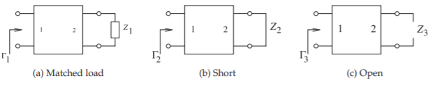
Figure \(\PageIndex{1}\): Two-port error network with three different calibration loads.

the device under test (DUT). All that is needed to determine the parameters of a two-port are three precisely known loads.

Calibration of the measurement system is critical, as the effect of cabling and connectors can be more significant than that of the device being measured. The process of removing the effect of cabling and connectors is called de-embedding. Ideally, perfect short, open, and matched loads would be available, but these can only be approximated, and numerous schemes have been developed for alternative ways of calibrating an RF measurement system. In some cases, for example, in measuring integrated circuits using what is called on-wafer probing, it is very difficult to realize a good match. A solution is to use calibration standards that consist of combinations of transmission line lengths and repeatable reflections. These calibration procedures are known mostly by combinations of the letters T, R, and L such as through-reflect-line TRL [3] (which relies on a transmission line of known characteristic impedance to replace the match); or through-line (TL), [4, 5] (which relies on symmetry to replace the third standard).

4.3.1 One-Port Calibration

In one-port measurements the desired reflection coefficient cannot be obtained directly. Instead, there is effectively an error network between the measurement plane at the load and the ideal internal network analyzer port. The network model [6] of the measurement system is shown in Figure \(\PageIndex{1}\) together with three ideal calibration standards. Calibration, here, is concerned with determining the \(S\) parameters of the error two-port.

Various calibration schemes have been developed, some of which are better in particular measurement environments, such as when measuring on-chip structures. Calibration schemes share certain commonalities. One of these is that the errors can be represented as a two-port (or several two-ports) that exists between an effective reference plane internal to the measurement equipment and the reference plane at the device to be measured. This device is commonly called the device under test (DUT). Known standards are placed at the device reference plane and measurements are made. The concept is illustrated by considering the determination of the \(S\) parameters of the two-port shown in Figure \(\PageIndex{1}\). With \(Z_{1}\) being a matched load, the input reflection coefficient \(\Gamma_{1}\) is \(S_{11}\):

\[\label{eq:1}S_{11}=\Gamma_{1} \]

The other commonly used calibration loads are \(Z_{2} = 0\) (a short circuit) and \(Z_{3} =\infty\) (an open circuit). In calibration precision shorts and opens are

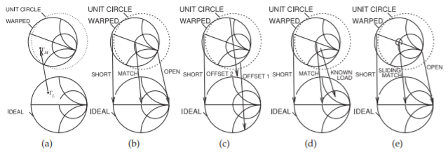
Figure \(\PageIndex{2}\): Calibrations as mapping operations with each calibration mapping having a warped Smith chart and an ideal Smith chart. The raw measurement of a reflection coefficient of a load is not the actual reflection coefficient, \(\Gamma_{L}\), but instead is the raw measurement, \(\Gamma_{M}\), which appears on a Smith chart that is warped (see (a)). In calibration, the raw measurements of standards also appear on the warped Smith chart although their actual values are known: (b) calibration as a mapping established using short, match, and open calibration standards; (c) mapping using short and two offset short calibration standards; (d) mapping using a short, a match, and a known load as calibration standards; and (e) mapping using a short, an open, and a sliding matched load as calibration standards.

are used and the errors involved are known and incorporated in the more detailed calibration procedure. From these, \(S_{12} = S_{21}\) and \(S_{22}\) can be derived:

\[\label{eq:2}S_{22}=\frac{2S_{11}-\Gamma_{2}-\Gamma_{3}}{\Gamma_{2}-\Gamma_{3}} \]

and

\[\label{eq:3}S_{21}=S_{12}=[(\Gamma_{3}-S_{11})(1-S_{22})]^{\frac{1}{2}} \]

The error two-port modifies the actual reflection coefficient of a DUT to a warped (but calibrated) reflection coefficient according to Equation (3.2.12). In Equation (3.2.12), the load reflection coefficient, \(\Gamma_{L}\), is a complex number that is scaled, rotated, and shifted before being presented at \(\Gamma_{\text{in}}\). Moreover, circles of reflection coefficient are mapped to circles on the warped complex plane; that is, the ideal Smith chart is mapped to a warped Smith chart. Here the actual load reflection coefficient, \(\Gamma_{L}\), is warped to present a measured reflection coefficient, \(\Gamma_{M}\) to the internal network analyzer. Calibration can be viewed as a mapping operation from the complex plane of raw measurements to the complex plane of ideal measurements, as shown in Figure \(\PageIndex{2}\)(a). That is, calibration develops the required mapping. Figure \(\PageIndex{2}\)(b–e) shows how the corrected mapping is developed using different sets of calibration standards. The mapping operation shown in Figure \(\PageIndex{2}\)(b) uses the short, open, and match loads. This one-port calibration procedure is called open-short-load or SOL calibration and is available as a calibration algorithm in all network analyzers. The three standards are well distributed over the Smith chart and so the mapping can be extracted with good precision. While ideal short, open, and match loads are not available, if the terminations are well characterized then appropriate corrections can be made. The mapping in the one-port case is embodied in the extracted \(S\)

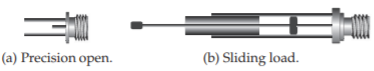
Figure \(\PageIndex{3}\): Precision calibration standards.

parameters of the two-port.

Figure \(\PageIndex{3}\)(a) shows the longitudinal section of a precision coaxial open. The key feature is that the outer coaxial conductor is extended and the fringing capacitance at the end of the center conductor can be calculated analytically. Thus the precision open is not a perfect open, but rather an open that can be modeled as a small capacitor whose frequency variation is known. Figure \(\PageIndex{2}\)(c) uses offset shorts (i.e., short-circuited transmission lines of various lengths). This circumvents the problem of difficult-to-produce open and matched loads. Care is required in the choice of offsets to ensure that the mapping can be determined accurately. The calibration scheme shown in Figure \(\PageIndex{2}\)(d) introduces a known load. The mapping cannot be easily extracted here, but in some situations this is the only option. Figure \(\PageIndex{2}\)(e) introduces a new concept in calibration with the use of a sliding matched load such as that shown in Figure \(\PageIndex{3}\)(b). A perfect matched load cannot be produced and there is always, at best, a small resistance error and perhaps parasitic capacitance. When measured, the reflection will have a small offset from the origin. If the matched load is moved, as with a sliding matched load, a small circle centered on the origin will be traced out and the center of this circle is the ideal matched load.

4.3.2 De-Embedding

The one-port calibration described above can be repeated for two ports, resulting in the two-port error model of Figure \(\PageIndex{4}\)(a), the error model for correcting two-port measurements. Using the chain scattering matrix (or \(\mathbf{T}\) matrix\(^{1}\)) introduced in Section 2.6, the \(\mathbf{T}\) parameter matrix measured at the internal reference planes of the network analyzer is

\[\label{eq:4}\mathbf{T}_{\text{MEAS}}=\mathbf{T}_{A}\mathbf{T}_{\text{DUT}}\mathbf{T}_{B} \]

where \(\mathbf{T}_{A}\) is the \(\mathbf{T}\) matrix of the first error two-port, \(\mathbf{T}_{\text{DUT}}\) is the \(\mathbf{T}\) matrix of the device under test, and \(\mathbf{T}_{B}\) is the \(\mathbf{T}\) matrix of the right-hand error two-port. Manipulating Equation \(\eqref{eq:4}\) leads to \(\mathbf{T}_{\text{DUT}}\):

\[\begin{align}\label{eq:5}\mathbf{T}_{A}^{-1}\mathbf{T}_{\text{MEAS}}\mathbf{T}_{B}^{-1}&=\mathbf{T}_{A}^{-1}\mathbf{T}_{A}\mathbf{T}_{\text{DUT}}\mathbf{T}_{B}\mathbf{T}_{B}^{-1}\\ \label{eq:6}\mathbf{T}_{\text{DUT}}&=\mathbf{T}_{A}^{-1}\mathbf{T}_{\text{MEAS}}\mathbf{T}_{B}^{-1}\end{align} \]

from which the \(S\) parameters of the DUT can be obtained.

4.3.3 Two-Port Calibration

The VNA architecture introduced in 1968 and still commonly used today is shown in Figure 4.2.1. A key component of the system is the test set that comprises mechanical microwave switches and directional couplers that selectively couple energy in either the forward- or backward-traveling waves. Many modern VNAs use multiple mixers and electronic switches to

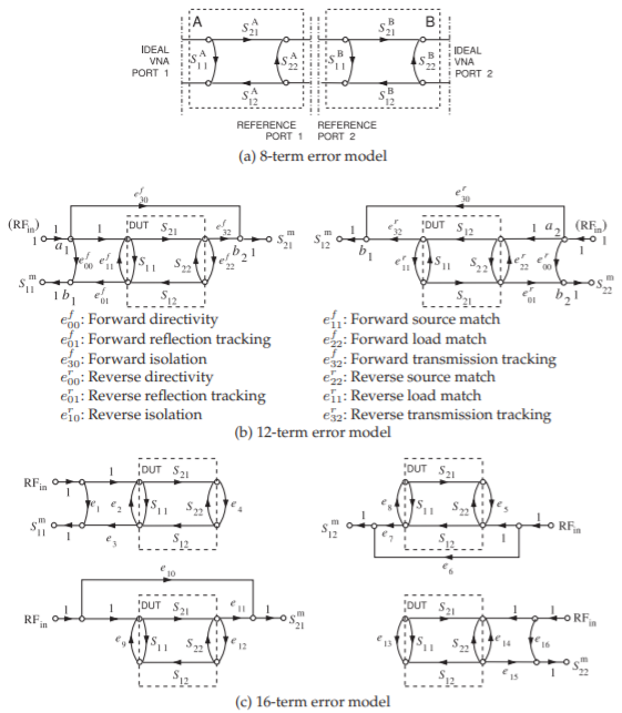
Figure \(\PageIndex{4}\): Two-port error models: (a) SFG representation of the 8-term two-port error model (1968) [1]); (b) SFG of the 12-term two-port error model (1978) [7]; and (c) SFG of the 16- term two-port error model (circa 1979) [8]. \(S_{ij}^{m}\) are the raw \(S\) parameter measurements, \(S_{ij}\) are the \(S\) parameters of the DUT, and \(e_{ij}\), \(e_{ij}^{r}\), and \(e_{ij}^{f}\) are error \(S\) parameters determined during calibration.

eliminate the need for mechanical switches. Operation is similar. Returning to the architecture of Figure 4.2.1, this architecture supports a single signal source and a single test port at which the RF signal to be measured is mixed down to a low frequency, typically \(100\text{ kHz}\), where it is captured by an ADC. The mixing component is called the frequency converter, and it mixes the RF signal with a version of the original RF signal offset in frequency to produce a low-frequency version of the RF signal. This has the same phase as the RF signal and an amplitude that is linearly proportional to the RF signal. When Hackborn introduced this system in 1968 [1], he also introduced the 8-term error model shown in Figure \(\PageIndex{4}\)(a). This is an extension of the one-port error model discussed in Section 4.3.1, with a two-port capturing the measurement errors to each port.

Closer examination of the VNA system of Figure 4.2.1 indicates that the signal path varies for each of the four scattering parameters for a DUT. Another imperfection that is not immediately obvious is that there is leakage in the system so that Ports \(\mathsf{1}\) and \(\mathsf{2}\) are coupled by a number of mechanisms that do not involve transmission of the signal through the DUT. Leakage is due to finite isolation in the mixers and direct coupling between probes used to make contact at Ports \(\mathsf{1}\) and \(\mathsf{2}\), among other possible causes. The first person to identify this was Shurmer [9] in 1973, leading eventually to the 12-term error model [7, 10] shown in Figure \(\PageIndex{4}\)(b). Calibration yields the error parameters, and the \(S\) parameters of the DUT are found as follows:

\[\begin{align}\label{eq:7}S_{11}&=\frac{1}{\delta}\left\{\left[\frac{S_{11}^{m}-e_{00}^{f}}{e_{01}^{f}}\right]\left[1+\frac{S_{22}^{m}-e_{00}^{r}}{e_{01}^{r}}e_{22}^{r}\right]-e_{22}^{f}\left[\frac{S_{21}^{m}-e_{30}^{f}}{e_{32}^{f}}\right]\left[\frac{S_{12}^{m}-e_{10}^{r}}{e_{32}^{r}}\right]\right\} \\ \label{eq:8}S_{21}&=\frac{1}{\delta}\left\{\left[\frac{S_{21}^{m}-e_{30}^{f}}{e_{32}^{f}}\right]\left[1+\frac{S_{22}^{m}-e_{00}^{r}}{e_{01}^{r}}\left(e_{22}^{r}-e_{22}^{f}\right)\right]\right\} \\ \label{eq:9}S_{12}&=\frac{1}{\delta}\left\{\left[\frac{S_{12}^{m}-e_{10}^{r}}{e_{32}^{r}}\right]\left[1+\frac{S_{11}^{m}-e_{00}^{f}}{e_{01}^{f}}\left(e_{11}^{f}-e_{11}^{r}\right)\right]\right\} \\ \label{eq:10}S_{22}&=\frac{1}{\delta}\left\{\left[\frac{S_{22}^{m}-e_{00}^{r}}{e_{01}^{r}}\right]\left[1+\frac{S_{11}^{m}-e_{00}^{f}}{e_{01}^{f}}e_{11}^{f}\right]-e_{11}^{r}\left[\frac{S_{21}^{m}-e_{30}^{f}}{e_{32}^{f}}\right]\left[\frac{S_{12}^{m}-e_{10}^{r}}{e_{32}^{r}}\right]\right\} \\ \delta&=\left[1+\frac{S_{11}^{m}-e_{00}^{f}}{e_{01}^{f}}e_{11}^{f}\right]\left[1+\frac{S_{22}^{m}-e_{00}^{r}}{e_{01}^{r}}e_{22}^{r}\right] \\ \label{eq:11}&\quad -e_{22}^{f}e_{11}^{r}\left[\frac{S_{21}^{m}-e_{30}^{f}}{e_{32}^{f}}\right]\left[\frac{S_{12}^{m}-e_{10}^{r}}{e_{32}^{r}}\right]\end{align} \]

The most complete model is the 16-term error model introduced in 1979 and shown in Figure \(\PageIndex{4}\)(c), which incorporates a different model for each parameter and fully captures the various signal paths resulting from the different switch positions [8]. Nevertheless, the 12-term error model is the one most commonly used in microwave measurements and is sufficient to reliably extract the desired \(S\) parameters of the DUT from the raw VNA measurements. This process of extracting the de-embedded parameters is call de-embedding, or less commonly, unterminating.

The 12-term error model models the error introduced by leakage or crosstalk internal to the network analyzer. The 16-term error model captures the leakage or crosstalk of the 12-term error model, but in addition includes switch leakage that results in error signals reflecting from the DUT and leaking to the transmission port as well as common-mode leakage [11]. This method is called two-port 16-term singular value decomposition (SVD) calibration, as the equations are solved in a least squares sense using the singular value decomposition method [11]. In a coaxial environment, the extra leakage terms are small, provided that the switches have high isolation. However, in wafer probing where direct coupling between the probes can be appreciable, the transmission-related leakage can be important and the 16- term error model captures errors that the 12-term error model does not. These error models and the sequence of measurements to extract them are included in the VNA control software. The user must select which to use.

Coaxial Two-Port Calibration

If the DUT has coaxial connectors then precision open, short, and matched loads are available. While these are not ideal components, the open has fringing capacitance; for example, they are well characterized over frequency. The full set of standards required to develop the 12-term error model includes one-port measurements for each port with open, short, and match connections, a two-port measurement with a through connection, and a two-port measurement with opens at each port. The last measurement determines the internal isolation of the system. Most connectors come in male and female counterparts. As such it is not possible to create a perfect through by joining the connectors and a small delay is introduced. There are, however, sexless connectors, such as the Amphenol precision connector (APC-7) with a \(7\text{ mm}\) outer diameter as it has a flush face that can be connected for a near-perfect through. The APC-7 connector is no longer commonly used, with most coaxial systems now using SMA connectors or the higher-tolerance APC 3.5 connectors that come in male and female connectors. The majority of the measurements desired these days are of ICs and other planar structures for which there is no clear connector. The connector, or fixture, problem has resulted in a variety of standards being used.

Planar Circuit Calibration

Calibration standards are required in microwave measurements. For measurements of microstrip and CPW systems, standard calibration alumina substrates are available, see Figure 4.2.5(d and e). These calibration substrates include various lengths of transmission lines that can be used as standards, as well as an open, a short, and a laser-trimmed matched load.

4.3.4 Transmission Line-Based Calibration Schemes

A drawback of all de-embedding techniques that use repeated fixture measurements during the de-embedding process is the generation of errors caused by the lack of fixture reproducibility during measurements of each of the required standards. These errors can be amplified during the course of de-embedding.

The TRL technique [3] is a calibration procedure used for microwave measurements when classical standards such as open, short, and matched terminations cannot be realized. There are now a family of related techniques, here denoted as TxL methods, with the commonality being the two-port measurement of a through connection and of the same structure with an inserted transmission line. The two-port connections required in the TRL procedure are shown in Figure \(\PageIndex{5}\). The concept behind the representation is that there is a measurement error that is captured by

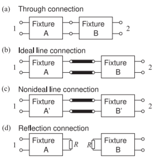
Figure \(\PageIndex{5}\): Measurement connections in two-port calibration using the TRL procedure: (a) through connection; (b) ideal line connection; (c) realistic configuration with nonidentical fixtures; and (d)with arbitrary reflection.

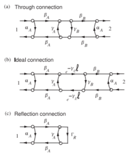
Figure \(\PageIndex{6}\): SFG representations of the twoport connections shown in Figure \(\PageIndex{5}\): (a) through connection; (b) ideal line connection; and (c) arbitrary reflection connection.

the fixture two-port. The TRL procedure allows the fixtures on either side, Fixtures A and B here, to have different two-port parameters. The SFG representations of the connections are shown in Figure \(\PageIndex{6}\). Assuming that the fixtures are faithfully reproduced when going from one connection to another, then the SFGs shown in \(\PageIndex{6}\)(a–c) need to be considered. With each configuration, two-port measurements are made, and as the number of independent \(S\) parameter measurements exceed the number of unknowns, it would seem that it may be possible to solve the SFGs to obtain the unknown parameters of the fixtures. This is all that is required to de-embed measurements made with a DUT between the fixtures. Unfortunately this is not possible. However, Engen and Hoer [3] developed a procedure that enabled the complex propagation constant of the line to be extracted from the external \(S\) parameter measurements of the through and line connections. This procedure is considered in the next section.

4.3.5 Through-Line Calibration

The through and line measurement structures include fixtures as well as the direct connection (for the through) and the inserted line (for the line) (see Figure \(\PageIndex{5}\)). Two-port measurements of these two structures yield the propagation constant \(\Gamma_{L} = \alpha +\jmath\beta\) of the line [3]. Similar but earlier work was presented by Bianco et al. [12]. For the through structure, the error networks between the ideal internal port of a network analyzer and the desired measurement reference plane are designated as Fixture \(\mathsf{A}\) at Port \(\mathsf{1}\) and Fixture \(\mathsf{B}\) at Port \(\mathsf{2}\). For the line measurement, fixturing is reestablished (following the through measurement) with the line inserted. In general, the fixturing cannot be faithfully reproduced and therefore becomes Fixtures \(\mathsf{A}′\) and \(\mathsf{B}′\), respectively (see Figure \(\PageIndex{5}\)).

The following is based on the derivation of Engen and Hoer [3]. As well as presenting an important result indicating sources of error in microwave measurement, the development demonstrates a technique for solving measurement problems involving transmission lines.

The development begins using cascading matrices, R, defined as

\[\label{eq:12}\left[\begin{array}{c}{b_{1}}\\{a_{1}}\end{array}\right]=\mathbf{R}\left[\begin{array}{c}{a_{2}}\\{b_{2}}\end{array}\right] \]

which is related to scattering parameters S by

\[\label{eq:13}\mathbf{R}=\left[\begin{array}{cc}{R_{11}}&{R_{12}}\\{R_{21}}&{R_{22}}\end{array}\right]=\left[\begin{array}{cc}{\frac{S_{12}S_{21}-S_{11}S_{22}}{S_{21}}}&{\frac{S_{11}}{S_{21}}} \\ {-\frac{S_{22}}{S_{21}}}&{\frac{1}{S_{21}}}\end{array}\right] \]

Thus the parameters describing the \(\mathsf{A}\) and \(\mathsf{B}\) fixtures are \(\mathbf{S}_{A},\: \mathbf{S}_{B}\) and \(\mathbf{R}_{A},\: \mathbf{R}_{B}\), respectively. The cascading matrix of the through is simply a unity matrix and the line of length, \(\ell_{L}\), is described by

\[\label{eq:14}\mathbf{R}_{L}=\left[\begin{array}{cc}{e^{-\gamma_{L}\ell_{L}}}&{0}\\{0}&{e^{\gamma_{L}\ell_{L}}}\end{array}\right] \]

The characteristic impedance of the line is taken as the reference impedance, \(Z_{0}\), of the measurement system and results in the off-diagonal zeros in the above definition for the line standard. Because of this simplifying assumption, \(\gamma_{L}\) can be computed using the equations that follow.

The cascading matrix of the through structure (i.e., the fixture-fixture cascade) is

\[\label{eq:15}\mathbf{R}_{t}=\mathbf{R}_{A}\mathbf{R}_{B}\quad\text{(the through)} \]

For the line structure, a fixturing error \(\Delta\) is introduced. \(\Delta\) corresponds to a small additional electrical length of the \(\mathsf{A}\) fixture (i.e., \(\mathbf{R}_{A}′ = \mathbf{R}_{A}\mathbf{R}_{e}\)), then the cascading matrix of the fixture-line-fixture cascade is

\[\label{eq:16}\mathbf{R}_{d} = \mathbf{R}'_{A}\mathbf{R}_{L}\mathbf{R}_{B} = \mathbf{R}_{A}\mathbf{R}_{e}\mathbf{R}_{L}\mathbf{R}_{B}\quad\text{(the line)}\quad\text{with}\quad\mathbf{R}_{e}=\left[\begin{array}{cc}{\text{e}^{-\Delta}}&{0}\\{0}&{\text{e}^{\Delta}}\end{array}\right] \]

Now introduce the matrix

\[\label{eq:17}\mathbf{T}=\left[\begin{array}{cc}{t_{11}}&{t_{12}}\\{t_{21}}&{t_{22}}\end{array}\right]=\mathbf{R}_{d}\mathbf{R}_{t}^{-1} \]

Thus \(\mathbf{T}\) combines the line and through measurements and approximately removes the through measurement from the line measurement. Most importantly, all of the elements of the \(\mathbf{T}\) matrix are measured quantities. Continuing (note that if \(\mathbf{A}\) and \(\mathbf{B}\) are matrices, \((\mathbf{AB})^{−1} = \mathbf{B}^{−1}\mathbf{A}^{−1}\)), and using Equations \(\eqref{eq:15}\)–\(\eqref{eq:17}\),

\[\begin{align}\mathbf{TR}_{A}&=\mathbf{R}_{d}\mathbf{R}_{t}^{−1}\mathbf{R}_{A} = \mathbf{R}'_{A} \mathbf{R}_{L}\mathbf{R}_{B}(\mathbf{R}_{A}\mathbf{R}_{B})^{−1}\mathbf{R}_{A}\nonumber \\ \label{eq:18}&=\mathbf{R}_{A}\mathbf{R}_{e}\mathbf{R}_{L}\mathbf{R}_{B}\mathbf{R}_{B}^{−1}\mathbf{R}_{A}^{−1}\mathbf{R}_{A}\end{align} \]

and so

\[\label{eq:19}\mathbf{TR}_{A}=\mathbf{R}_{A}\mathbf{R}_{e}\mathbf{R}_{L} \]

which is referred to as the TL (for through-line) equation. Expanding Equation \(\eqref{eq:19}\) leads to a system of equations:

\[\begin{align} \label{eq:20} t_{11}R_{A11} + t_{12}R_{A21} &= R_{A11}\text{e}^{−\Delta}\text{e}^{−\gamma_{L}\ell_{L}} \\ \label{eq:21} t_{21}R_{A11} + t_{22}R_{A21} &= R_{A21}\text{e}^{−\Delta}\text{e}^{−\gamma_{L}\ell_{L}} \\ \label{eq:22} t_{11}R_{A12} + t_{12}R_{A22} &= R_{A12}\text{e}^{\Delta}\text{e}^{\gamma_{L}\ell_{L}} \\ \label{eq:23} t_{21}R_{A12} + t_{22}R_{A22} &= R_{A22}\text{e}^{\Delta}e^{\gamma_{L}\ell_{L}} \end{align} \]

which upon solution yields the propagation constant of the line standard [3],

\[\begin{align}\label{eq:24}\gamma_{L}&=\frac{1}{2\ell_{L}}\left[\ln\left(\frac{t_{11}+t_{22}\pm\zeta}{t_{11}+t_{22}\mp\zeta}\right)-2\Delta\right] \\ \label{eq:25}\zeta&=(t_{11}^{2}-2t_{11} t_{22}+t_{22}^{2}+4t_{21}t_{12})^{1/2}\end{align} \]

If the fixtures are faithfully reproduced, then networks \(\mathsf{A}\) and \(\mathsf{A}'\) are identical, as are networks \(\mathsf{B}\) and \(\mathsf{B}'\), and so \(\Delta=0\), and \(\gamma_{L}\) is

\[\label{eq:26}\gamma_{L}=\frac{1}{2\ell_{L}}\ln\left(\frac{t_{11}+t_{22}\pm\zeta}{t_{11}+t_{22}\mp\zeta}\right) \]

The sign to use with \(\zeta\) is chosen corresponding to the root selection [3].

That is, two-port \(S\) parameter measurements of the through connection (shown in Figure \(\PageIndex{5}\)(a)) and two-port \(S\) parameter measurements of the line connection (shown in Figure \(\PageIndex{5}\)(b)) enable the propagation constant of the line to be determined. The characteristic impedance of the line standard can be determined as described in Section 4.5.

Extraction of the propagation constant of the transmission line standard is a common property of calibration techniques that use through and line measurements instead of match measurements. Such techniques are called TxL techniques, where \(\text{x}\) identifies an additional measurement used in calibration. Unfortunately the TxL calibration techniques often result in errors in de-embedding at frequencies where the length of the line standard is a multiple of one-half wavelength (called critical lengths [13, 14]). These are the lengths where the electrical length is a multiple of \(180^{\circ}\). Buff et al. [15, 16] showed that small fixture repeatability errors result in errors incorporated in \(\Delta\). These errors affect the entire calibration and subsequent de-embedded measurements. These errors are minimized by using measurements where the line standard has an electrical length not within \(20^{\circ}\) of a critical length. Statistical means and the use of multiple lines have been proposed to minimize the error [17, 18], as well as an optimization scheme to determine the additional electrical length, \(\Delta\) [15, 16]. The optimization scheme significantly reduces the uncertainty and is based on the assumption that a change of line length is the sole source of error in fixture reproducibility (the fixture here includes, of course, the probe and probe pad). This is seen in Figure \(\PageIndex{7}\) where the results of optimization are seen most clearly for the attenuation constant in Figure \(\PageIndex{7}\)(a), the curve labeled fixture error de-embedded. The no fixture error curve was selected as the best results from a large number of calibrations (multiple repeats of probe-on-probe pad connections). The fixture error curve is the result of a typical calibration measurement.

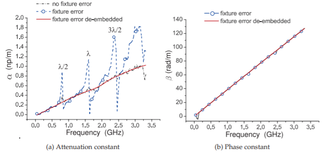
Figure \(\PageIndex{7}\): Extracted propagation constant from the through and line components of TRL with fixture error introduced during the line measurement.

In the following, several of the TxL calibration techniques are described. These are techniques incorporated in most vector network analyzers and are particularly useful in characterizing on-chip circuits. An example of an on-wafer two-port measurement is shown in Figure \(\PageIndex{8}\), showing on-chip calibration standards. The VNA software leads the user through the required set of calibration measurements and computes the error models to be used in de-embedding.

Through Short Delay

Matched loads can be difficult to realize, especially when probing ICs and planar circuits using probes. The through short delay (TSD) method uses reflection and transmission measurements [19]. The delay is realized using a line with a \(50\:\Omega\) characteristic impedance. TSD experiences the \(180^{\circ}\) glitches common to TxL schemes. The through could be another delay, but then problems occur when the delay difference (the electrical length difference) of the through and delay is an integer multiple of \(180^{\circ}\).

Through Reflect Line

What has become known as the through reflect line (TRL) calibration technique was developed by Bianco et al. [12] and Engen and Hoer [3], who used a through connection, an arbitrary reflection standard, and a delay or line standard. The line standard can be of arbitrary length with its propagation constant unknown, but it is assumed to be nonreflecting. The result of this assumption is that the characteristic impedance of the line becomes the system reference impedance. Also, the reflection standard, can be any repeatable reflection load, with an open or short preferred. Again the transmission line introduces calibration uncertainties when the electrical

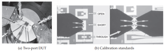
Figure \(\PageIndex{8}\): Two-port measurements: (a) two-port device under test with DC needle probes at the bottom and GSG probes on the left and right; and (b) open, short, and through calibration standards with GSG probes.

length is a multiple of one-half wavelength [3].

Through Reflect Match

Through reflect match (TRM) is a variation of TRL that replaces the through by a matched load and is useful only when a matched load can be realized. It retains the arbitrary reflection standard, which is particularly useful as it can be difficult to produce a short or open with planar circuits. For example, a via used in realizing a microstrip short circuit has finite resistance and inductance and so does not create a good through, but does create a useful repeatable arbitrary reflection. The technique does not have the critical length glitches, but repeatable fixturing is always important.

Other Distributed Calibration Techniques

TRL and TRM are the most commonly accepted standards used in calibrating measurements of planar circuit structures. There are several other related techniques that also use transmission lines and are useful in certain circumstances.

In 1982 Benet [20] developed the open-short-five-offset-line calibration technique. The key concept is that the multiple offset through lines trace out a circle on the Smith chart and the center of the circle provide the matched load. Through least squares fitting Benet derived the propagation constant of the through lines and the remaining error terms to develop the 12-term error model.

Pennock et al. [21] introduced the double through line (DTL) calibration system in 1987. This is useful for characterizing transitions between different mediums. There is sufficient information to develop the 6-term error model. SOLT (short-open-load-through) calibration requires precisely characterized standards and is robust to \(20\text{ GHz}\).

SOLR (short-open-load-reciprocal-through) calibration is similar to SOLT using precisely defined reflect standards as a standard.

LRRM, (line-reflect-reflect-match) calibration uses a line instead of a through, one of the reflection standards is a short and the other is an open. This is

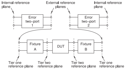
Figure \(\PageIndex{9}\): Two-tier calibration procedure.

usually the best calibration technique to use with probes, as these standards are straightforward to incorporate in calibration substrates. The calibration standards are the same as those used in SOLT, but LRRM does not require precision short and open standards. The essentials of what must be known are the characteristics of the through and the DC resistance of one of the load standards. The inductance of the load is automatically determined.

LRM, (load-reflect-match) calibration is similar to LRRM calibration but does not use a precision reflect standard. A modification is LRM+, for which the DC resistances of the loads are required.

4.3.6 Two-Tier Calibration

With measurements in noncoaxial systems, it is difficult to produce precision standards such as shorts, opens, and resistive loads. In these situations, two-tier calibration is sometimes used. In a two-tier calibration procedure, two sets of standards are used to establish first- and second-tier reference planes (see Figure \(\PageIndex{9}\)). It is preferable to use a highly repeatable set of standards in Tier \(\mathsf{1}\) (such as a non-TxL technique), and one that yields more precise characterization in a particular environment (such as a TxL technique for on-wafer measurement).

In the first-tier calibration, a precision set of standards is normally used. This can be achieved using coaxial standards or perhaps a standard calibration substrate used with probes. Referring to Figure \(\PageIndex{9}\), each of the \(\mathsf{2}\) two-ports from the internal reference planes of the network analyzer to the external reference planes is established. Generally with the second tier, insitu calibration standards are used, and the additional (e.g. on-chip) fixturing is identical for the two ports. Precision calibration should be done using standards fabricated in the medium of the DUT.

Two-tier calibration generally results in the fixtures in the second tier being identical. This enables checks to be made for the integrity of the probe connection. Connections to IC pads can be problematic because of oxide build up, especially with aluminum pads. So ensuring symmetry of second-tier calibrations by comparing the two-port measurements of symmetrical structures such as transmission lines can greatly reduce the impact of the fixture-induced errors discussed in Section 4.3.5. Recall that small fixturing errors, such as bringing the probes down in slightly different positions,

Figure \(\PageIndex{10}\): Measurement connections in two-port second-tier calibration using the TL calibration procedure: (a) through connection; (b) ideal line connection; (c) realistic configuration showing that the fixtures are not precisely reproduced; and (d) arbitrary reflection configuration.

results in measurement errors at the half-wavelength frequencies (\(\lambda/2,\:\lambda,\: 3\lambda /2,\) etc.). For example, if the DUT is a device on a silicon wafer, the optimum measurement technique is to realize the calibration standards on the silicon wafer processed in the same way as for the DUT. The two-tier calibration procedure removes fixturing errors associated with fringing effects at the probes and with other nonidealities involved in creating the landing pads for the probes.

In an example two-tier calibration scheme, a first tier is used to establish the 12-term error model. Then a second calibration is used to develop a secondary six-term error model, as in Figure \(\PageIndex{4}\)(a) with \(S_{12} = S_{21}\). In such a situation the standards used in developing the 12-term error model would normally include an open, a short, and a matched load. These need not be precise standards. Thus the 12-term error model need not be precise, and this model does not suffer from the half-wavelength errors of the TxL techniques.

Through Line Symmetry

For planar measurements using probes, first-tier calibration using a standard calibration substrate is to the end of the probe tips, and errors with using other substrates (e.g., the probe pads are of different size or the substrate permittivity is different) will be common to both probes (fixtures) in a two-port measurement. With careful design, the fixtures employed in the second tier will be identical and have the same \(S\) parameters. In the second-tier calibration, measurements of a through and line will be symmetrical with \(S_{11} = S_{22}\) and \(S_{12} = S_{21}\). This symmetry is exploited in the through line (TL) technique which exploits symmetry and renders the half-wavelength errors of TxL insignificant [4, 5]. The TL calibration connections in second-tier calibration are shown in Figure \(\PageIndex{10}\). In the first calibration tier, a 12-term error model is developed using open, short, load, and delay. Consequently there are no half-wavelength glitches that occur when transmission line standards are used. In the second calibration tier, probes are used with two lengths of transmission line fabricated on the same substrate as the DUT. One of the lines becomes a through.

The procedure proceeds by calculating the propagation constant of the line using the technique developed for the TRL procedure (Equation \(\eqref{eq:26}\)). There is fixture symmetry in the TL connections (see Figure \(\PageIndex{10}\)) and this is reflected in the SFG representations of the connections as shown in Figure \(\PageIndex{11}\). As will be shown, this symmetry enables the arbitrary reflection used

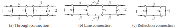
Figure \(\PageIndex{11}\): SFG representations of the two-port connections shown in Figure \(\PageIndex{10}\).

in the TRL procedure to be replaced by a virtual precise short or open circuit. Let the \(S\) parameters of Fixture \(\mathsf{A}\) be \(\alpha = S_{11},\:\beta = S_{12} = S_{21}\), and \(\gamma = S_{22}\). Using these parameters with the port reversal required to model the Fixture at Port \(\mathsf{2}\), the SFG shown in Figure \(\PageIndex{11}\)(a) relates the measured \(S\) parameters to the parameters of the fixtures. The input reflection coefficient of Fixture \(\mathsf{A}\) with a short circuit placed at Port \(\mathsf{2}\) of \(\mathsf{A}\) is

\[\label{eq:27}\rho_{\text{sc}}=\alpha-\frac{\beta^{2}}{1+\gamma} \]

Let the measured \(S\) parameters of the through connection be designated by a leading superscript \(T\). Using the self-loop (or Mason’s) rule with the SFG in Figure \(\PageIndex{11}\)(a) relates the measured \(S\) parameters to the fixture parameters:

\[\label{eq:28}^{T}S_{11}=\alpha+\frac{\beta^{2}\gamma}{1-\gamma^{2}}\quad\text{and}\quad\:^{T}S_{21}=\frac{\beta^{2}}{1-\gamma^{2}} \]

Subtracting these expressions yields

\[\begin{align}^{T}S_{11}-\:^{T}S_{21}&=\alpha+\frac{\beta^{2}\gamma}{1-\gamma^{2}}-\frac{\beta^{2}}{1-\gamma^{2}}=\alpha+\frac{\beta^{2}\gamma-\beta^{2}}{(1-\gamma)(1+\gamma)}\nonumber \\ \label{eq:29}&=\alpha-\frac{\beta^{2}(1-\gamma)}{(1-\gamma)(1+\gamma)}=\alpha-\frac{\beta^{2}}{1+\gamma}=\rho_{\text{sc}}\end{align} \]

That is, the input reflection coefficient of a fixture terminated in a virtual ideal short circuit can be obtained from the through measurement of the back-to-back fixtures in the through configuration:

\[\label{eq:30}\rho_{\text{sc}}=\:^{T}S_{11}-\:^{T}S_{21} \]

Similar results are obtained for a virtual ideal open circuit placed at Port \(\mathsf{2}\) of Fixture \(\mathsf{A}\):

\[\label{eq:31}\rho_{\text{oc}}=\:^{T}S_{11}+\:^{T}S_{21} \]

Thus it is possible to effectively insert ideal open and short circuits within a noninsertable medium.

Footnotes

[1] Note that there are several \(\mathbf{T}\) matrices, so it necessary to be specific.