5.13: Transmission Line-Based Hybrids

Hybrids can be realized in a variety of transmission line structures. A few of these, but representative ones, are discussed here. Hybrids can also be realized using lumped-elements by modeling the transmission line segments.

5.13.1 Branch-Line Hybrids Based on Transmission Lines

A branch-line hybrid is based on transmission line segments that introduce phase delay. Two such hybrids are shown in Figure 5.12.10 where the different signal paths result in constructive and destructive interference of signals. This is a very different way of realizing the hybrid function than that obtained using magnetic transformers. The operation of the \(180^{\circ}\) hybrid (Figure 5.12.10(a)) can be verified approximately by counting the total number of one-quarter wavelength \((90^{\circ})\) phase shifts in each path. It is not so easy to verify the operation of the \(90^{\circ}\) hybrid. The various characteristic impedances of the transmission line segments adjust the levels of the signals. The operation of the \(90^{\circ}\) hybrid is examined in the example in this section. (A complete analysis could be done using signal flow graphs.)

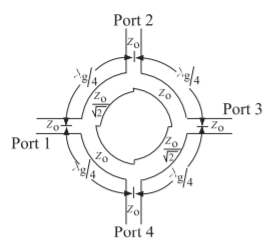
Figure \(\PageIndex{1}\): Planar implementation of the \(3\text{ dB}\) ring-type branch-line hybrid with the topology of Figure 5.12.10(b).

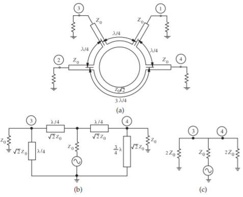
Figure \(\PageIndex{2}\): Rat-race hybrid with input at Port \(\mathsf{1}\), outputs at Ports \(\mathsf{3}\) and \(\mathsf{4}\), and virtual ground at Port \(\mathsf{2}\): (a) implementation as a planar circuit; (b) transmission line model; and (c) equivalent circuit model.

These branch-line hybrids may be formed into a ring shape, as shown in Figure \(\PageIndex{1}\). It is also worth considering the so-called rat-race or hybrid-ring circuit shown in Figure \(\PageIndex{2}\)(a). Output signals from Ports \(\mathsf{2}\) and \(\mathsf{4}\) differ in phase by \(180^{\circ}\) (in contrast to the branch-line coupler, where the phase difference is \(90^{\circ}\)). An interesting and important design feature arises when considering the quarter-wave transformer action of this coupler. Only Ports \(\mathsf{2}\) and \(\mathsf{4}\) exhibit this action, because Port \(\mathsf{3}\) is half-wave separated from the input feeding Port \(\mathsf{1}\). Thus the net effective load on the inner ring lines feeding Ports \(\mathsf{2}\) and \(\mathsf{4}\) amounts to \(2Z_{0}\) (two \(Z_{0}\) loads appearing, equivalently, in series). Now the characteristic impedance \(Z_{0}\) of any quarter-wave transforming line between two impedances, \(Z_{01}\) and \(Z_{02}\), is equal to \(\sqrt{Z_{01}Z_{02}}\). In this case the two impedances are \(Z_{0}\) and \(2Z_{0}\), respectively, so (from Section 2.4.6 of [15]) the input impedance of the intervening quarter-wave line is

\[\label{eq:1} Z_{0}'=\sqrt{Z_{0}\cdot 2Z_{0}}=\sqrt{2}Z_{0} \]

Thus the characteristic impedance of the line forming the ring itself is \(\sqrt{2}\) times that of the feeder line impedances. So when the impedance of all ports is \(50\:\Omega\), the ring characteristic impedance is \(70.7\:\Omega\).

Exercise \(\PageIndex{1}\): Rat-Race Hybrid

In this example the rat-race circuit shown in Figure \(\PageIndex{2}\)(a) is considered. One of the functions of this circuit is that with an input at Port \(\mathsf{1}\), the power of this signal is split between Ports \(\mathsf{3}\) and \(\mathsf{4}\). At the same time, no signal appears at Port \(\mathsf{2}\). This example is an exercise in exploiting the impedance transformation properties of the transmission line.

From Figure \(\PageIndex{2}\)(a) it is seen that each port is separated from the other port by a specific electrical length. Intuitively one can realize that there will be various possible outputs for excitation from different ports. Each case will be studied.

When Port \(\mathsf{1}\) of the hybrid is excited or driven, the outputs at Ports \(\mathsf{3}\) and \(\mathsf{4}\) are in phase, as both are distanced from Port \(\mathsf{1}\) by an electrical length of \(\lambda_{g}/4\), while Port \(\mathsf{2}\) remains isolated, as the electrical length of the two paths from Port \(\mathsf{1}\) to Port \(\mathsf{2}\) differ by an even multiple of \(\lambda_{g}/2\). Thus Port \(\mathsf{2}\) will be an electrical short circuit to the signal at Port \(\mathsf{1}\).

In a similar way, a signal excited at Port \(\mathsf{2}\) will result in outputs at Ports \(\mathsf{3}\) and \(\mathsf{4}\), though with a phase difference of \(180^{\circ}\) between the two output ports and Port \(\mathsf{1}\) remains isolated.

Finally, a signal excited at Ports \(\mathsf{3}\) and \(\mathsf{4}\) will result in the sum of the two signals at Port \(\mathsf{1}\) and the difference of two signals at Port \(\mathsf{2}\). This combination of output is again due to varying electrical length between every port and every other port in the rat-race hybrid. The equivalent transmission line model and equivalent circuit of the rat-race hybrid are shown in Figures \(\PageIndex{2}\)(b and c), respectively.

5.13.2 Lumped-Element Hybrids

Hybrids are developed based on transmission line principles, but it is possible to create hybrids using lumped-element equivalents of transmission line segments. In some cases the full circle of design can begin with the magnetic transformer conceptualization, followed by a transmission line realization, and then a lumped-element approximation. At least this is valid over a bandwidth centered at a particular frequency, \(f = \omega_{0}/(2\pi )\). The lumped-element equivalent of the \(180^{\circ}\) hybrid in Figure 5.12.10(a) is shown in Figure \(\PageIndex{3}\)(a) with

\[\label{eq:2}\omega_{0}L=\frac{1}{\omega_{0}C}=\sqrt{2}Z_{0} \]

This result comes from the broadband equivalent circuit of a \(\lambda /4\) line shown in Figure 2-37. The lumped-element quadrature hybrid of Figure \(\PageIndex{3}\)(b), based on Figure 5.12.10(b), has

\[\label{eq:3}\omega_{0}Z_{0}C_{a}=1,\quad C_{a}+C_{b}=\frac{1}{\omega_{0}^{2}L},\quad\text{and}\quad \omega_{0}L=\frac{Z_{0}}{\sqrt{2}} \]

where \(Z_{0}\) is the port impedance.

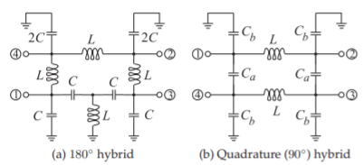
Figure \(\PageIndex{3}\): Lumped-element hybrids.