5.9: Hybrids

Hybrids are transformers that combine or divide microwave signals among a number of inputs and outputs. They can be implemented using distributed or lumped elements and are not restricted to RF and microwave applications. For example, a magnetic transformer is a hybrid and can be used to combine the outputs of two or more transistor stages, or to obtain appropriate impedance levels. A \(3\text{ dB}\) directional coupler based on parallel coupled lines is also a type of hybrid. Specific implementations will be considered later in this chapter, but for now the focus is on their idealized characteristics. The symbols commonly used for hybrids are shown in Figure 5.8.2.

A hybrid is a special type of four-port junction with the property that if a signal is applied at any port, it emerges from two of the other ports at half power, while there is no signal at the fourth or isolated port. The two outputs have specific phase relationships and all ports are matched. Only two fundamental types of hybrids are used: \(180^{\circ}\) and \(90^{\circ}\) hybrids. A hybrid is a type of directional coupler, although the term directional coupler, or just coupler, is most commonly used to refer to devices where only a small fraction of the power of an input signal is sampled. Also, a balun is a special type of hybrid.

5.9.1 Quadrature Hybrid

The ideal \(90^{\circ}\) hybrid, or quadrature hybrid, shown in Figure 5.8.2(c), has the scattering parameters

\[\label{eq:1}S_{90^{\circ}}=\frac{1}{\sqrt{2}}\left[\begin{array}{cccc}{0}&{-\jmath}&{1}&{0}\\{-\jmath}&{0}&{0}&{1}\\{1}&{0}&{0}&{-\jmath}\\{0}&{1}&{-\jmath}&{0}\end{array}\right] \]

The \(90^{\circ}\) phase difference between the through and coupled ports is indicated by \(−\jmath\). The actual phase shift, that is, \(+90^{\circ}\) or \(−90^{\circ}\) (indicated by \(\jmath\)), between the input and output ports depends on the specific hybrid implementation. Another quadrature hybrid could have the parameters

\[\label{eq:2}S_{90^{\circ}}=\frac{1}{\sqrt{2}}\left[\begin{array}{cccc}{0}&{\jmath}&{1}&{0}\\{\jmath}&{0}&{0}&{1}\\{1}&{0}&{0}&{\jmath}\\{0}&{1}&{\jmath}&{0}\end{array}\right] \]

Recall the requirement of quadrature modulators that the local oscillator be supplied as two components equal in magnitude but \(90^{\circ}\) out of phase. A quadrature hybrid is just the circuit that can do this.

To convince yourself that Equation \(\eqref{eq:2}\) describes a network that splits the power, consider the power flow implied by Equation \(\eqref{eq:2}\). The fraction of power transmitted from Port \(i\) to Port \(j\) is described by \(|S_{ji}|^{2}\). Consider the power that enters Port \(\mathsf{1}\). No power is reflected for an ideal hybrid, as the input at Port \(\mathsf{1}\) is matched and \(S_{11} = 0\). Port \(\mathsf{4}\) should be isolated so no power will come out of Port \(\mathsf{4}\), and so \(S_{41} = 0\). The power should be split between Ports \(\mathsf{2}\) and \(\mathsf{3}\), and these should be equal to half the power entering Port \(\mathsf{1}\). From Equation \(\eqref{eq:2}\),

\[\label{eq:3}|S_{21}|^{2}=\left(\frac{1}{\sqrt{2}}|j|\right)^{2}=\frac{1}{q}\quad\text{and}\quad |S_{31}|^{2}=\left(\frac{1}{\sqrt{2}}|1|\right)^{2}=\frac{1}{2} \]

Thus the power entering Port \(\mathsf{1}\) is split, with half going to Port \(\mathsf{2}\) and half to Port \(\mathsf{3}\).

5.9.2 \(180^{\circ}\) Hybrid

The scattering parameters of the \(180^{\circ}\) hybrid, shown in Figure 5.8.2(b), are

\[\label{eq:4}S_{180^{\circ}}=\frac{1}{\sqrt{2}}\left[\begin{array}{cccc}{0}&{1}&{-1}&{0}\\{1}&{0}&{0}&{1}\\{-1}&{0}&{0}&{1}\\{0}&{1}&{1}&{0}\end{array}\right] \]

and this defines the operation of the hybrid. In terms of the root power waves \(a\) and \(b\), the outputs at the ports are

\[\label{eq:5}\begin{array}{ll} {b_{1}=(a_{2}-a_{3})/\sqrt{2}}&{b_{2}=(a_{1}+a_{4})/\sqrt{2}}\\{b_{3}=(-a_{1}+a_{4})/\sqrt{2}}&{b_{4}=(a_{2}+a_{3})/\sqrt{2}}\end{array} \]

Imperfections in fabricating the hybrid will result in nonzero scattering parameters at the ports where ideally \(S_{ji} = 0\), so that it is best to terminate

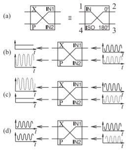
Figure \(\PageIndex{1}\): A \(180^{\circ}\) hybrid as a combiner (with output at the sum port, \(\sum\)) and as a comparator (with output at the difference port, \(\Delta\)): (a) equivalence between a \(180^{\circ}\) hybrid and a sum-and-difference hybrid; (b) the two inputs are in phase; (c) the two inputs are \(180^{\circ}\) out of phase; and (d) the two inputs are \(90^{\circ}\) out of phase.

the isolated port of the hybrid, as shown in Figure 5.8.2(d), to ensure that there is no reflected signal (i.e., no \(a_{4}\)) entering the hybrid at the isolated port. Equation \(\eqref{eq:5}\) shows that ports are interchangeable. That is, if a signal is applied to Port \(\mathsf{3}\), then it is split between Ports \(\mathsf{1}\) and \(\mathsf{4}\), and Port \(\mathsf{2}\) becomes the isolated port.

A hybrid can be used in applications other than splitting the input signal into a through and a coupled component. An example of another use is in a system that combines or compares two signals, as in Figure \(\PageIndex{1}\). Here a \(180^{\circ}\) hybrid with the scattering parameters of Equation \(\eqref{eq:4}\) is shown. With a signal \(x(t)\) applied to Port \(\mathsf{2}\) in Figure 5.8.2(b), and another signal \(y(t)\) applied to Port \(\mathsf{3}\), the output at Port \(\mathsf{4}\) is the sum signal, \(x(t) + y(t)\), and the output at Port \(\mathsf{1}\) is the difference signal, \(x(t) − y(t)\). More common names for the output ports (when the \(180^{\circ}\) hybrid is used as a combiner) are to call Port \(\mathsf{4}\) the sigma or sum port, often designated using the symbol \(\sum\). Port \(\mathsf{1}\) is called the difference or delta port, \(\Delta\). Notice that if a signal is applied to the \(\Delta\) port it will generate out-of-phase outputs.

5.9.3 Magnetic Transformer Hybrid

In the hybrid circuits of Figures \(\PageIndex{2}\) and \(\PageIndex{3}\), the number of windings of each coil (there are three in each structure) is the same. The impedance levels given are those required for maximum power transfer and indicate the impedance transformations of the structures. Considering Figure \(\PageIndex{3}\) and equating powers,

\[\label{eq:6}\frac{1}{2}\frac{(2V)^{2}}{Z_{2}}=\frac{1}{2}\frac{V^{2}}{Z_{0}},\quad\frac{4}{Z_{2}}=\frac{1}{Z_{0}}\quad\text{and so}\quad Z_{2}=4Z_{0} \]

That is, if \(Z_{2} = 4Z_{0}\), the impedance seen looking into Port \(\mathsf{4}\) (of the transformer in Figure \(\PageIndex{3}\)) is \(Z_{0}\), and so the transformer has provided matching to the large load. For example, if \(Z_{2} = 200\:\Omega\) (perhaps the input of a transistor), the transformer matches this to \(50\:\Omega\).

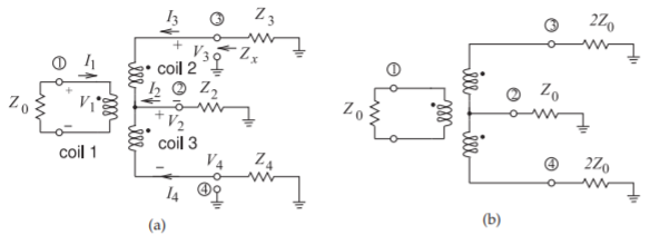
Figure \(\PageIndex{2}\): Magnetic transformer hybrid with each coil having the same number of windings: (a) showing general loading impedance; and (b) optimum loading to function as a \(180^{\circ}\) hybrid with Port \(\mathsf{2}\) (terminal \(\mathsf{2}\) to ground) isolated and the balanced input at Port \(\mathsf{1}\). For example, an antenna could be attached to Port \(\mathsf{1}\). A common flux passes through the three coils.

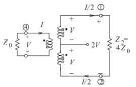
Figure \(\PageIndex{3}\): The magnetic transformer of Figure \(\PageIndex{2}\) as an impedance transforming balun.

Example \(\PageIndex{1}\): Magnetic Transformer Hybrid

Consider the magnetic transformer hybrid of Figure \(\PageIndex{2}\)(a) with \(Z_{0}\) real. Determine what type of hybrid this is and calculate the impedance transformations. Assume ideal coupling \((k = 1)\).

Solution

Since the coupling is ideal and each coil has the same number of windings,

\[\label{eq:7}(V_{3}-V_{2})=V_{1}\quad\text{and}\quad (V_{2}-V_{4})=V_{1} \]

The current levels in the transformer depend on the attached circuitry. For this circuit to function as a hybrid with Port \(\mathsf{2}\) isolated, the current \(I_{2}\) must be zero so that \(I_{3}\) and \(I_{4}\) are equal in magnitude but \(180^{\circ}\) out of phase. The loading at Ports \(\mathsf{3}\) and \(\mathsf{4}\) must be the same. Now \(V_{2} = 0,\) since \(I_{2} = 0,\) and so Equation \(\eqref{eq:7}\) become

\[\label{eq:8}V_{3}=V_{1}\quad\text{and}\quad V_{4}=-V_{1} \]

so this circuit is a \(180^{\circ}\) hybrid.

To determine loading conditions at Ports \(\mathsf{2,}\) \(\mathsf{3,}\) and \(\mathsf{4}\) the following transformer equation is used:

\[\label{eq:9}V_{3}=\jmath\omega L_{2}I_{3}+\jmath\omega MI_{1}-\jmath\omega MI_{4} \]

where \(L_{2}\) is the inductance of Coil \(\mathsf{2}\) and \(M\) is the mutual inductance. Now \(I_{1} = −V_{1}/Z_{0},\: L_{2} = L_{3} = M\) since coupling is ideal, and \(V_{3} = V_{1}\). So Equation \(\eqref{eq:9}\) becomes

\[\label{eq:10}V_{3}=\jmath\omega M(2I_{3}-V_{3}/Z-{0})\quad\text{That is,}\quad V_{3}(1+\jmath\omega M/Z_{0})=\jmath 2\omega MI_{3} \]

If \(\jmath\omega M≫|Z_{0}|,\) this reduces to

\[\label{eq:11}Z_{x}=V_{3}/I_{3}=2Z_{0} \]

For maximum power transfer \(Z_{3} = Z_{x}^{\ast}\), but since \(Z_{0}\) is real, \(Z_{3} = Z_{x} = 2Z_{0}\). From symmetry, \(Z_{4} = Z_{3}\). Also, \(I_{3} = −I_{4} = I_{1}/2\).

(The above result can also be obtained by considering only maximum power transfer considerations. The argument is as follows. An impedance \(Z_{0}\) is attached to Coil \(\mathsf{1}\). Maximum power transfer to the transformer through the coil requires that the input impedance be \(Z_{0}\) (since it is real). In the ideal hybrid operation the power is split evenly between the powers delivered to the loads at Ports \(\mathsf{3}\) and \(\mathsf{4}\), since \(V_{1} = (V_{3} − V_{2})=(V_{2} − V_{4})\) and the power delivered to Coil \(\mathsf{1}\) is \(V_{1}^{2}/(2Z_{0})\). The power delivered to \(Z_{3}\) (and \(Z_{4}\)) is \((V_{3} − V_{2})^{2}/(2Z_{3}) = V_{1}^{2}/(2Z_{3}) = V_{1}^{2}/(4Z_{0})\). That is, \(Z_{3} = 2Z_{0} = Z_{4}\). It is a small extrapolation to say that \(Z_{3} = 2Z_{0}^{\ast}= Z_{4}\).)

The problem is not yet finished, as \(Z_{2}\) must be determined. For hybrid operation, a signal applied to Port \(\mathsf{2}\) should not have a response at Port \(\mathsf{1}\). So the current at Port \(\mathsf{2},\: I_{2},\) should be split between Coils \(\mathsf{2}\) and \(\mathsf{3}\) so that \(I_{3} = −I_{2}/2 = I_{4}\). Thus

\[\label{eq:12}V_{4}=-I_{4}(2Z_{0})=(I_{2}/2)(2Z_{0})=I_{2}Z_{0}=V_{3} \]

Now

\[\label{eq:13}V_{3} − V_{2} = V_{1} =0= V_{2} − V_{4},\quad\text{and so}\quad V_{2} = V_{4} = I_{2}Z_{0} \]

That is,

\[\label{eq:14}Z_{2}=V_{2}/I_{2}=Z_{0} \]

The final \(180^{\circ}\) hybrid circuit is shown in Figure \(\PageIndex{2}\)(b) with the loading conditions for matched operation as a hybrid.

In the example above it is seen that the number of windings in the coils are the same so that the current in Coils \(\mathsf{2}\) and \(\mathsf{3}\) (of the transformer in Figure \(\PageIndex{2}\)) is half that in Coil \(\mathsf{1}\). The general rule is that with an ideal transformer, the sum of the amp-turns around the magnetic circuit must be zero. The precise way the sum is calculated depends on the direction of the windings indicated by the “dot” convention. A generalization of the rule for the transformer shown in Figure \(\PageIndex{2}\) is

\[\label{eq:15}n_{1}I_{1}-n_{2}I_{2}-n_{3}I_{3}=0 \]

where \(n_{j}\) is the number of windings of Coil \(j\) with current \(I_{j}\). The example serves to illustrate the type of thinking behind the development of many RF circuits. Considering maximum power transfer provided an alternative, simpler start to the solution of the problem than one that used the full transformer equations.