6.8: Distributed Matching

Matching using lumped elements leads to series and shunt lumped elements. The shunt elements can be implemented using shunt transmission lines, as a short length (less than one-quarter wavelength long) of short-circuited transmission line looks like an inductor and a short section of open-circuited transmission line looks like a capacitor. However, in most transmission line technologies it is not possible to realize the series elements as lengths of transmission lines. While it has been shown that a short length of transmission line is inductive, replacing series inductors by a length of transmission line of high characteristic impedance is not the best approach to realizing networks. The solution is to use lengths of transmission line together with shunt elements. If space is not at a premium, this is an optimum solution, as transmission lines have much lower loss than a lumped inductor. The series transmission lines rotate the reflection coefficient on the Smith chart.

As with all matching design, using transmission lines begins with a topology in mind. Several topologies are shown in Figure \(\PageIndex{1}\). Figure \(\PageIndex{1}\)(a) is the

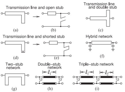
Figure \(\PageIndex{1}\): Matching networks with transmission line elements.

top view of a microstrip matching network with a series transmission line and stub realized as an open-circuited transmission line. Figure \(\PageIndex{1}\)(b) is a shorthand schematic for this circuit. Matching network design then becomes a problem of choosing the lengths and characteristic impedances of the lines. The stub here is used to realize a capacitive shunt element. This network corresponds to two-element matching with a shunt capacitor. The value of the shunt capacitance can be increased using a dual stub, as shown in Figure \(\PageIndex{1}\)(c), where the capacitive input impedances of each stub are in parallel. The dual circuit to that in Figure \(\PageIndex{1}\)(a) is shown in Figure \(\PageIndex{1}\)(d) together with its schematic representation in Figure \(\PageIndex{1}\)(e). This circuit has a short-circuited stub that realizes a shunt inductance.

Mixing lumped capacitors with a transmission line element, as shown in Figure \(\PageIndex{1}\)(f), realizes a much more space-efficient network design. There are many variations to stub-based matching network design, including the two-stub design in Figure \(\PageIndex{1}\)(g).

A common situation encountered in the laboratory is the matching of circuits that are in development. Laboratory items available for matching include the stub tuner, shown in Figure \(\PageIndex{2}\)(a), and the double-stub tuner, shown in Figure \(\PageIndex{2}\)(b). With the double-stub tuner the length of the series transmission line is fixed, but stubs can have variable length using lengths of transmission lines with sliding short circuits. Not all impedances can be matched using a double stub tuner, however. A triple-stub tuner can match all impedances presented to it [2]. The double-slug tuner shown in Figure \(\PageIndex{2}\)(c) has dielectric slugs each of which introduces a short section of lower impedance line. The slugs are moved up and down the line and avoid the rapid changes in impedances that occur with the stub tuners and as a result the double-slug tuner provides a broader bandwidth match than does the double stub tuner. The slide-screw slug tuner shown in Figure \(\PageIndex{2}\)(d) can achieve a broadband match. Here a metal slug can be lowered into the slabline changing the impedance of a section of transmission line and mostly affects the magnitude of the reflection coefficient while moving the metal slug along the line mostly affects the phase. This is the type of tuner incorporated in computer-controlled automated tuners.

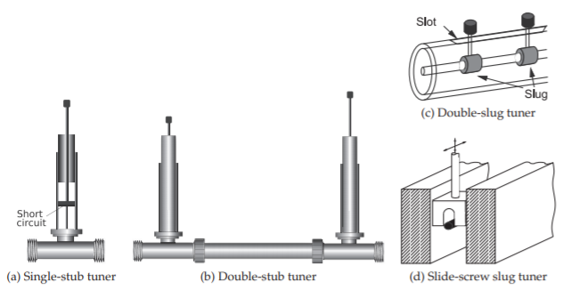
Figure \(\PageIndex{2}\): Laboratory tuners.

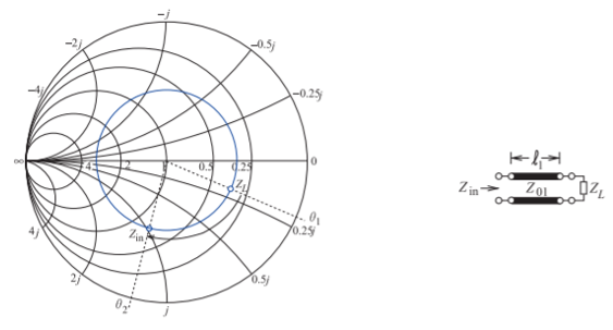
Figure \(\PageIndex{3}\): Rotation of the input impedance of a transmission line on a Smith chart normalized to \(Z_{01}\) as the line length increases.

6.8.1 Stub Matching

In this section matching using one series transmission line and one stub will be considered. This corresponds to the microstrip circuit topologies shown in Figures \(\PageIndex{1}\)(a and d). First, consider the terminated transmission line shown in Figure \(\PageIndex{3}\). When the length, \(\ell_{1}\), of the line is zero, the input impedance of the line, \(Z_{\text{in}}\), equals \(Z_{L}\). How it changes is best described by considering the input reflection coefficient, \(\Gamma_{\text{in}}\), of the line. If the reflection coefficient is normalized to \(Z_{01}\), then the magnitude of \(\Gamma_{\text{in}}\) and its phase varies as twice the electrical length of the line. This situation is shown on the Smith chart in Figure \(\PageIndex{3}\), where \(Z_{L}\) is chosen arbitrarily. The input reflection coefficient of

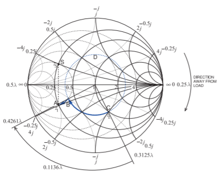
Figure \(\PageIndex{4}\): Design for Example \(\PageIndex{1}\).

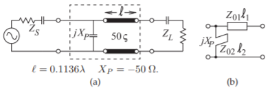
Figure \(\PageIndex{5}\): Single-stub matching network design of Example \(\PageIndex{1}\): (a) electrical design; and (b) electrical design with a shunt stub.

the line rotates in a clockwise direction as the length of the line increases. One way of remembering this is to consider an open-circuited line. When the line length is zero, \(Y_{\text{in}} = 0\) and \(\Gamma_{\text{in}} = +1\). A short length of this line is capacitive so that its reflection coefficient will be in the bottom half of the Smith chart. A length of line can be used to rotate the impedance to an appropriate point to follow a line of constant conductance to the desired input impedance.

Example \(\PageIndex{1}\): Matching Network Design With a Transmission Line and a Single Stub

Design a two-element matching network to match a source with an impedance \(Z_{S} = 12.5 + 12.5\jmath\:\Omega\) to a load \(Z_{L} = 50 − 50\jmath\:\Omega\), as shown in Figure 6.7.5. This example repeats the design in Example 6.7.2, but now using a transmission line.

Solution

As in Example 6.7.2, choose \(Z_{0} = 50\:\Omega\) and the design path is from \(z_{L} = Z_{L}/Z_{0} = 1−\jmath\) to \(z_{s}^{\ast}\), where \(z_{s} = 0.25 + 0.25\jmath\). One possible design solution is indicated in Figure \(\PageIndex{4}\). The line length, \(\ell\) (taking the locus from Point \(\mathsf{C}\) to Point \(\mathsf{B}\)), is

\[\ell=0.4261\lambda -0.3125\lambda =0.1136\lambda\nonumber \]

and the normalized shunt susceptance, \(b_{P}\) (taking the locus from Point \(\mathsf{B}\) to Point \(\mathsf{C}\)), is

\[b_{P}=b_{A}-b_{B}=2-1=1 \nonumber \]

Thus \(X_{P} = (−1/b_{P} )\times 50\:\Omega = −50\:\Omega\). The final design is shown in Figure \(\PageIndex{5}\)(a). The stub design of Figure \(\PageIndex{5}\)(b) follows the procedure described in Example 6.5.1.

6.8.2 Hybrid Lumped-Distributed Matching

A lossless matching network can have transmission lines as well as inductors and capacitors. If the system reference or normalization impedance is the characteristic impedance of a transmission line, then the locus of the input impedance (or reflection coefficient) of the line with respect to the length of the line is an arc on a circle centered at the origin of the Smith chart. The direction of the arc is clockwise as the electrical length of the line moves away from the load. So a hybrid matching network is possible that combines a length of transmission line with a lumped element (preferably a capacitor rather than an a inductor as the inductor would have a relatively lower \(Q\)).