7.7: Broadband Matching to Reactive Loads

Previous sections presented methods for broadband matching to resistive loads. Usually these techniques work quite well if the load is moderately reactive but this is not always the case. Inputs and outputs of transistors can have larger reactive parts than resistive parts. Broadband matching to such loads requires customization taking into account the frequency locus of the loads which nearly always rotates in the clockwise direction on a Smith chart so that the locus of the complex conjugate match rotates in the counterclockwise direction. Circuits that achieve broadband match to these loads exploit resonance and as such have limited bandwidths so that half-octave matching is usually the most that can be achieved.

7.7.1 Broadband Matching to a Series RC Load

Consider matching to the input of a transistor. A transistor such as a FET has an input that can be modeled as a capacitor in series with a resistor as shown in Figure \(\PageIndex{1}\)(a). At \(10\text{ GHz}\) the \(294\text{ fF}\) capacitor has a reactance of \(−54.06\:\Omega\) so that the \(Q\) of the load is \(2.36\). The Fano-Bode limit, see Equation (7.2.7), indicates that the maximum fractional bandwidth that can be achieved

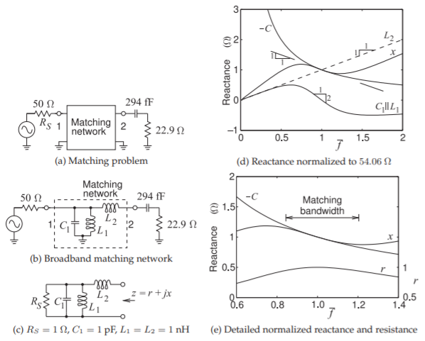
Figure \(\PageIndex{1}\): Broadband matching with normalized frequency \(\overline{f}\) in radians/s normalized to \(10\text{ GHz}\).

for an average reflection coefficient, \(\Gamma_{\text{avg}}\), at Port \(1\) of \(0.11\) is \(60\%\). This \(\Gamma_{\text{avg}}\) corresponds to an average transmission loss of \(0.05\text{ dB}\) for a maximum transmission loss of approximately \(0.1\text{ dB}\) in the bandwidth of the match.

Note

Note that if the load was purely resistive, then \(Q = 0\) and it is theoretically possible to achieve infinite bandwidth.

Matching would be greatly simplified if the matching network presented a negative capacitor to the load. The reactance normalized to \(54.06\:\Omega\) versus frequency of the required negative capacitance (of capacitance \(−294\text{ fF}\)) is shown as the curve identified as \(−C\) in Figure \(\PageIndex{1}\)(d). At the normalized frequency \(\overline{f} = 1\) (frequency normalized to \(10\text{ GHz}\)) the slope of this curve is \(−1\). A circuit that approximates this over a moderate bandwidth is the broadband matching network shown in Figure \(\PageIndex{1}\)(b). To see how this is achieved, consider the input impedance of the circuit in Figure \(\PageIndex{1}\)(c).

The reactance of the parallel \(\text{LC}\) subcircuit is shown in Figure \(\PageIndex{1}\)(d) as the curve labeled \(C_{1}\parallel L_{1}\). At \(\hat{f} = 1\) this reactance has a slope of \(−2\) and adding a series inductor, \(L_{2}\), (having the reactance curve \(L_{2}\) in Figure \(\PageIndex{1}\)(d)) results in a reactance \(x\), see Figure \(\PageIndex{1}\)(d), which does have a slope of \(−1\) at \(\hat{f} = 1\). Thus the total reactance, \(x\), closely matches the reactance of a negative capacitor over a limited, but still broad, bandwidth. The other part

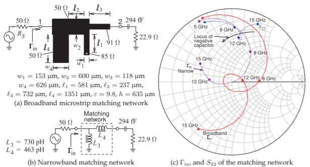
Figure \(\PageIndex{2}\): Broadband and narrowband matching networks with \(\Gamma_{\text{in}}\) of both networks and \(S_{22}\) of the broadband network shown with the the locus of the ideal conjugate match (identified as the locus of negative capacitor). In (a) \(\ell_{1} = 0.048\lambda,\:\ell_{2} = 0.020\lambda,\:\ell_{3} = 0.060\lambda,\) and \(\ell_{4} = 0.117\lambda\) at \(10\text{ GHz}\). In (b) a \(50\:\Omega\) Smith chart is used.

of the matching problem is matching the source and load resistances and with appropriate choice of matching network values the resistance \(r\) (ideally \(22.9\:\Omega\) normalized to \(54.06\:\Omega\)) will be approximately constant in the matching region, see Figure \(\PageIndex{1}\)(e).

A microstrip realization centered at \(10\text{ GHz}\) of the broadband matching network concept is shown in Figure \(\PageIndex{2}\)(a). At Port \(\mathsf{1}\) is an open-circuited stub with a relatively short electrical length at \(10\text{ GHz}\) and so presents the capacitance \(C_{1}\). This is followed by a short section of line that separates the two stubs and provides an extra degree of freedom to be used in matching the source and load resistances. Then follows a short shorted stub that implements \(L_{1}\). This is followed by a short high-impedance line which introduces the series inductance \(L_{2}\) (see Section 2.4.5 of [6]). The performance of the matching network is shown in Figure \(\PageIndex{2}\)(c) where it is compared to that of a narrowband matching network. The narrowband network, shown in Figure \(\PageIndex{2}\)(b), is a conventional two-element matching network designed using the absorption method so that the \(294\text{ fF}\) capacitor is absorbed into the network but still requires an additional inductance \(L_{4}\) to compensate for the capacitance. The match of both the broadband and narrowband matching networks is ideal at \(10\text{ GHz}\). The \(\Gamma_{\text{in}}\) loci of the two networks are shown on a \(50\:\Omega\) Smith chart in Figure \(\PageIndex{2}\)(c).

The range of match for a maximum transmission loss of \(0.1\text{ dB}\) is from \(9.04\text{ GHz}\) to \(11.53\text{ GHz}\) (a \(2.49\text{ GHz}\) bandwidth) for the broadband network and \(9.47\text{ GHz}\) to \(10.62\text{ GHz}\) (a \(1.15\text{ GHz}\) bandwidth) for the narrowband network. Using a \(0.5\text{ dB}\) bandwidth criterion the bandwidth of the region of match for the broadband microstrip network is \(8.13\text{ GHz}\) to \(12.95\text{ GHz}\) (a \(4.82\text{ GHz}\) bandwidth) and the narrowband network has a passband from \(8.54\text{ GHz}\) to \(12.34\text{ GHz}\) (a \(3.80\text{ GHz}\) bandwidth).

Also plotted in Figure \(\PageIndex{2}\)(c) is \(S_{22}\) of the broadband microstrip network and from this the reason why a good match is achieved can be seen. Typically the reflection coefficient locus of simple networks rotates clockwise on the Smith chart with increasing frequency. For a small frequency range near the center match frequency \(S_{22}\) has a loop and effectively rotates in the counterclockwise direction approximating the locus of a negative capacitor. Such a behavior is obtained in the lumped element version of the broadband network by the resonance of \(L_{1},\: C_{1},\) and \(L_{2}\). A very good match is therefor possible over a small frequency range. The good match is obtained over about half an octave (of frequency) and this is typically the best that can be achieved when matching to the inputs and outputs of microwave transistors. The microstrip broadband matching network has a finite length and width. Including the widths as well as the lengths of the lines, the broadband matching network has a width and length of \(0.11\:\lambda\), considerably less than that of a quarter-wave transformer used to match resistive source and load impedances when they are resistive but not when the load has a large reactance as here.

7.7.2 Summary

The broadband matching concept presented in this section is using resonance to present an impedance to a load or source that rotates in the counterclockwise direction (with respect to frequency) on a Smith chart. This is achievable only over a moderate bandwidth and typically half-octave bandwidths are regarded as the limit of what can be achieved when matching to a load that is more reactive than resistive. There are techniques also that are sometimes able to achieve broader effective matches by incorporating the parasitic reactances of a device to be matched into a distributed transmission line.