
2.9: Coaxial Line
- Page ID
- 41023

\( \newcommand{\vecs}[1]{\overset { \scriptstyle \rightharpoonup} {\mathbf{#1}} } \)
\( \newcommand{\vecd}[1]{\overset{-\!-\!\rightharpoonup}{\vphantom{a}\smash {#1}}} \)
\( \newcommand{\dsum}{\displaystyle\sum\limits} \)
\( \newcommand{\dint}{\displaystyle\int\limits} \)
\( \newcommand{\dlim}{\displaystyle\lim\limits} \)
\( \newcommand{\id}{\mathrm{id}}\) \( \newcommand{\Span}{\mathrm{span}}\)
( \newcommand{\kernel}{\mathrm{null}\,}\) \( \newcommand{\range}{\mathrm{range}\,}\)
\( \newcommand{\RealPart}{\mathrm{Re}}\) \( \newcommand{\ImaginaryPart}{\mathrm{Im}}\)
\( \newcommand{\Argument}{\mathrm{Arg}}\) \( \newcommand{\norm}[1]{\| #1 \|}\)
\( \newcommand{\inner}[2]{\langle #1, #2 \rangle}\)
\( \newcommand{\Span}{\mathrm{span}}\)
\( \newcommand{\id}{\mathrm{id}}\)
\( \newcommand{\Span}{\mathrm{span}}\)
\( \newcommand{\kernel}{\mathrm{null}\,}\)
\( \newcommand{\range}{\mathrm{range}\,}\)
\( \newcommand{\RealPart}{\mathrm{Re}}\)
\( \newcommand{\ImaginaryPart}{\mathrm{Im}}\)
\( \newcommand{\Argument}{\mathrm{Arg}}\)
\( \newcommand{\norm}[1]{\| #1 \|}\)
\( \newcommand{\inner}[2]{\langle #1, #2 \rangle}\)
\( \newcommand{\Span}{\mathrm{span}}\) \( \newcommand{\AA}{\unicode[.8,0]{x212B}}\)
\( \newcommand{\vectorA}[1]{\vec{#1}} % arrow\)
\( \newcommand{\vectorAt}[1]{\vec{\text{#1}}} % arrow\)
\( \newcommand{\vectorB}[1]{\overset { \scriptstyle \rightharpoonup} {\mathbf{#1}} } \)
\( \newcommand{\vectorC}[1]{\textbf{#1}} \)
\( \newcommand{\vectorD}[1]{\overrightarrow{#1}} \)
\( \newcommand{\vectorDt}[1]{\overrightarrow{\text{#1}}} \)
\( \newcommand{\vectE}[1]{\overset{-\!-\!\rightharpoonup}{\vphantom{a}\smash{\mathbf {#1}}}} \)
\( \newcommand{\vecs}[1]{\overset { \scriptstyle \rightharpoonup} {\mathbf{#1}} } \)
\( \newcommand{\vecd}[1]{\overset{-\!-\!\rightharpoonup}{\vphantom{a}\smash {#1}}} \)
\(\newcommand{\avec}{\mathbf a}\) \(\newcommand{\bvec}{\mathbf b}\) \(\newcommand{\cvec}{\mathbf c}\) \(\newcommand{\dvec}{\mathbf d}\) \(\newcommand{\dtil}{\widetilde{\mathbf d}}\) \(\newcommand{\evec}{\mathbf e}\) \(\newcommand{\fvec}{\mathbf f}\) \(\newcommand{\nvec}{\mathbf n}\) \(\newcommand{\pvec}{\mathbf p}\) \(\newcommand{\qvec}{\mathbf q}\) \(\newcommand{\svec}{\mathbf s}\) \(\newcommand{\tvec}{\mathbf t}\) \(\newcommand{\uvec}{\mathbf u}\) \(\newcommand{\vvec}{\mathbf v}\) \(\newcommand{\wvec}{\mathbf w}\) \(\newcommand{\xvec}{\mathbf x}\) \(\newcommand{\yvec}{\mathbf y}\) \(\newcommand{\zvec}{\mathbf z}\) \(\newcommand{\rvec}{\mathbf r}\) \(\newcommand{\mvec}{\mathbf m}\) \(\newcommand{\zerovec}{\mathbf 0}\) \(\newcommand{\onevec}{\mathbf 1}\) \(\newcommand{\real}{\mathbb R}\) \(\newcommand{\twovec}[2]{\left[\begin{array}{r}#1 \\ #2 \end{array}\right]}\) \(\newcommand{\ctwovec}[2]{\left[\begin{array}{c}#1 \\ #2 \end{array}\right]}\) \(\newcommand{\threevec}[3]{\left[\begin{array}{r}#1 \\ #2 \\ #3 \end{array}\right]}\) \(\newcommand{\cthreevec}[3]{\left[\begin{array}{c}#1 \\ #2 \\ #3 \end{array}\right]}\) \(\newcommand{\fourvec}[4]{\left[\begin{array}{r}#1 \\ #2 \\ #3 \\ #4 \end{array}\right]}\) \(\newcommand{\cfourvec}[4]{\left[\begin{array}{c}#1 \\ #2 \\ #3 \\ #4 \end{array}\right]}\) \(\newcommand{\fivevec}[5]{\left[\begin{array}{r}#1 \\ #2 \\ #3 \\ #4 \\ #5 \\ \end{array}\right]}\) \(\newcommand{\cfivevec}[5]{\left[\begin{array}{c}#1 \\ #2 \\ #3 \\ #4 \\ #5 \\ \end{array}\right]}\) \(\newcommand{\mattwo}[4]{\left[\begin{array}{rr}#1 \amp #2 \\ #3 \amp #4 \\ \end{array}\right]}\) \(\newcommand{\laspan}[1]{\text{Span}\{#1\}}\) \(\newcommand{\bcal}{\cal B}\) \(\newcommand{\ccal}{\cal C}\) \(\newcommand{\scal}{\cal S}\) \(\newcommand{\wcal}{\cal W}\) \(\newcommand{\ecal}{\cal E}\) \(\newcommand{\coords}[2]{\left\{#1\right\}_{#2}}\) \(\newcommand{\gray}[1]{\color{gray}{#1}}\) \(\newcommand{\lgray}[1]{\color{lightgray}{#1}}\) \(\newcommand{\rank}{\operatorname{rank}}\) \(\newcommand{\row}{\text{Row}}\) \(\newcommand{\col}{\text{Col}}\) \(\renewcommand{\row}{\text{Row}}\) \(\newcommand{\nul}{\text{Nul}}\) \(\newcommand{\var}{\text{Var}}\) \(\newcommand{\corr}{\text{corr}}\) \(\newcommand{\len}[1]{\left|#1\right|}\) \(\newcommand{\bbar}{\overline{\bvec}}\) \(\newcommand{\bhat}{\widehat{\bvec}}\) \(\newcommand{\bperp}{\bvec^\perp}\) \(\newcommand{\xhat}{\widehat{\xvec}}\) \(\newcommand{\vhat}{\widehat{\vvec}}\) \(\newcommand{\uhat}{\widehat{\uvec}}\) \(\newcommand{\what}{\widehat{\wvec}}\) \(\newcommand{\Sighat}{\widehat{\Sigma}}\) \(\newcommand{\lt}{<}\) \(\newcommand{\gt}{>}\) \(\newcommand{\amp}{&}\) \(\definecolor{fillinmathshade}{gray}{0.9}\)In this section the characteristic impedance of a coaxial line is calculated. The technique assumes that the dynamic electric and magnetic fields will be the same as they would be at DC. This physical insight enables the problem to be solved relatively simply using the static field laws. Later the dynamic situation is considered when the fields on a realistic coaxial line are considered.
2.9.1 Characteristic Impedance of a Coaxial Line
In the following the per unit length parameters—\(R,\: L,\: G,\) and \(C\)—of a coaxial line are obtained. From these the characteristic impedance and propagation constant of the coaxial line are derived. The development is an example of how these parameters can be developed for any transmission line. The key is using a coordinate system that matches the structure being considered. Then Maxwell’s equations can be expressed very simply, usually as one-dimensional ordinary differential equations. Very often the static electric and magnetic field laws can be used that make the development even simpler. If an orthogonal coordinate system does not coincide with the dimensions of the line, then sometimes it is possible to use a mathematical technique called conformal mapping to map a nonconforming shape such as a microstrip line into a shape that matches an orthogonal coordinate system [20]. Once the transmission line parameters are derived the result is mapped back to the original structure. Fortunately most transmission line structures conform to an orthogonal coordinate system.
The cross section of a coaxial line is shown in Figure \(\PageIndex{1}\)(a) and it has two concentric conductors with the inner conductor having an outer radius of \(a\) and the inside of the outer conductor with a radius \(b\). The fields between the conductors can be solved by expressing the field relations in cylindrical coordinates. The following is a simplification of the treatment in [21], which can be applied to a broader range of coaxial cables than just the circularly symmetrical conventional coaxial cable in Figure \(\PageIndex{1}\). The simplest possible field distribution is shown in Figure \(\PageIndex{1}\)(b). The first parameter to be developed is \(C\). For this, the charge on one of the conductors is related to the voltage between the conductors. Consider a section of line of length \(\Delta z\), then using Gauss’s law, Equation (1.6.6), the electric flux is related to the total charge enclosed. So at radius \(r\),
\[\begin{align} \oint_{s}\overline{D}&=Q_{\text{enclosed}}\nonumber \\ \label{eq:1} 2\pi rD_{r}(r)\Delta z&=\rho_{\ell}\Delta z\quad\text{and}\quad 2\pi r\varepsilon E_{r}(r)\Delta z=\rho_{\ell}\varepsilon\Delta z\end{align} \]
where \(\rho_{\ell}\) is the charge on the inner conductor per unit length (in the \(z\) direction). So the radial electric field is
\[\label{eq:2}\overline{E}=E_{r}(r)\hat{\mathbf{r}}=\frac{\rho_{\ell}}{2\pi r\varepsilon}\hat{\mathbf{r}} \]
and \(\mathbf{r}\) is the unit vector in the radial direction. The voltage between the conductors is
\[\label{eq:3}V=\int_{a}^{b}E_{r}\cdot dr=\int_{a}^{b}\frac{\rho_{\ell}}{2\pi r\varepsilon}\cdot dr=\frac{\rho_{\ell}}{2\pi\varepsilon}\ln\left(\frac{b}{a}\right) \]
Now, the total capacitance of a section of line is
\[\label{eq:4}C_{\text{TOTAL}}=C\Delta z=\frac{Q}{V}=\frac{\rho_{\ell}\Delta z}{V} \]
and so the capacitance per unit length of line is (with SI units of \(\text{F/m}\))
\[\label{eq:5}C=\frac{2\pi\varepsilon}{\ln(b/a)} \]
The conductance of the line is found beginning with the current density in the dielectric, which is
\[\label{eq:6}J=\sigma E+\jmath\omega\varepsilon E \]
Integrating this over the volume of the dielectric,
\[\label{eq:7}I=GV+\jmath\omega CV \]
Using a similar development to that which led to Equation \(\eqref{eq:5}\), the conductance per unit length is found to be (with the SI units of \(\text{S/m}\))
\[\label{eq:8}G=\frac{2\pi\sigma}{\ln(b/a)} \]
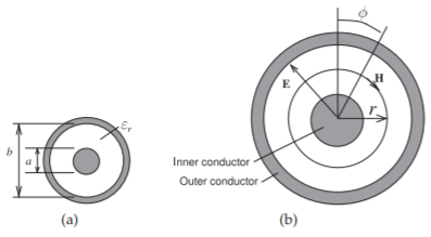
Figure \(\PageIndex{1}\): Coaxial line: (a) with inner an conductor of radius \(a\) and an outer conductor with inside radius \(b\); and (b) with cylindrical coordinates used in calculation.
The development of the expressions for \(L\) and \(R\) is more involved, as there will be current in the interior of the inner conductor. To simplify matters the high-frequency limit will be considered where the skin effect is fully established so that the currents on the inner and outer conductors are confined to a thin layer near the surfaces of the conductors at radius \(a\) for the inner conductor and at radius \(b\) for the outer conductor. Then the magnetic field will be confined to the region between the conductors. Using Ampere’s circuital law, Equation (1.6.1),
\[\label{eq:9}\oint_{\ell}\overline{H}\cdot d\ell =\oint_{\ell}H_{\phi}\hat{\mathbf{ϕ}}\cdot d\ell =I_{\text{enclosed}}=I \]
where the closed line integral is on a circle of constant radius. Noting that \(H_{r}\) is only a function of \(r\), then for \(a<r<b\),
\[\label{eq:10}I=2\pi r_{r}(r)\quad\text{and}\quad B_{r}=\mu H_{r}=\frac{\mu I}{2\pi r} \]
This enables the line inductance to be calculated as the total magnetic flux (obtained by integrating over the cross section of the coaxial line between radii \(a\) and \(b\)) per unit current. So the inductance of the line per unit length is
\[\label{eq:11}L=\int_{a}^{b}\left(\frac{\mu}{2\pi r}\right)dr=\frac{\mu}{2\pi}\ln\left(\frac{b}{a}\right) \]
which has SI units of \(\text{H/m}\).
The resistance of the lines is calculated using the surface resistance of the conductors, \(R_{s}\). So the resistance of the line per unit length is
\[\label{eq:12}R=\frac{R_{s}}{2\pi}\left(\frac{1}{a}+\frac{1}{b}\right) \]
which has the SI units of \(\Omega\text{/m}\).
Then the lossless characteristic impedance of the coaxial line is
\[\label{eq:13}Z_{0}=\sqrt{\frac{L}{C}}=\frac{1}{2\pi}\sqrt{\frac{\mu}{\varepsilon}}\ln\left(\frac{b}{a}\right) \]
which has units of \(\Omega\)s if all the quantities in the expression are in SI units. A complex characteristic impedance is derived using \(Z_{0} = \sqrt{(R + \jmath\omega L)/(G + \jmath\omega C)}\), but if the loss is small, this will be very close to the lossless characteristic impedance. Also
\[\label{eq:14}Z_{0}=\sqrt{\frac{\mu_{r}}{\varepsilon_{r}}}\frac{1}{2\pi}\sqrt{\frac{\mu_{0}}{\varepsilon_{0}}}\ln\left(\frac{b}{a}\right)=60\sqrt{\frac{\mu_{r}}{\varepsilon_{r}}}\ln\left(\frac{b}{a}\right) \]
Note that the \(60\) is exact and not an approximation.
For actual coaxial lines the dielectric has negligible loss and the resistance, \(R\), is small. Using the results developed in Section 2.5.4 for a low-loss line, the attenuation coefficient for a low-loss coaxial line is, from Equation (2.5.15),
\[\label{eq:15}\alpha\approx\alpha_{c}=\frac{R}{2Z_{0}}=\frac{R_{s}}{2\pi}\left(\frac{1}{a}+\frac{1}{b}\right)\frac{2\pi}{\ln(b/a)}\sqrt{\frac{\varepsilon}{\mu}}=\left(\frac{1}{a}+\frac{1}{b}\right)\frac{R_{s}}{\ln(b/a)}\sqrt{\frac{\varepsilon}{\mu}} \]
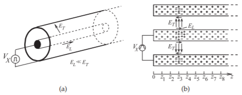
Figure \(\PageIndex{2}\): A coaxial transmission line: (a) three-dimensional view; (b) the line with pulsed voltage source showing the electric fields at an instant in time as a voltage pulse travels down the line.
which is the attenuation due to the conductor, that is, due to ohmic or conductor loss. From Equation \(\eqref{eq:15}\) it is seen that for a given characteristic impedance, and hence a fixed ratio \(b/a\), the attenuation coefficient and thus loss, is minimized when the line has a large cross section (i.e., large \(a\) and \(b\)). With a fixed \(a\), attenuation is minimized with \(b/a = 3.59\) independent of \(\mu\) and \(\varepsilon\) [17]. For an air-filled coaxial line with \(\mu_{r} =1= \varepsilon_{r}\), the characteristic impedance of this minimum-loss line is \(76.7\:\Omega\). For a typically Teflon-filled coaxial line \(\varepsilon_{r} = 2.1\) and the characteristic impedance of a minimum loss line, from Equation \(\eqref{eq:14}\), is \(52.9\:\Omega\). The above result is when the conductivity of the inner and outer conductors is the same and the internal inductance of the conductors is negligible. If the internal inductance is not negligible, or the conductors have different conductivity, which happens when the conductors are not solid, then the optimum characteristic impedance could be higher or lower [17]. The choice of \(50\:\Omega\) for the characteristic impedance is a good compromise. Other optimum line dimensions can be derived for maximizing breakdown voltage and optimizing power transfer [22].
The upper operating frequency and dimensions of coaxial lines are chosen to ensure single-mode propagation [23, 24, 25]. A useful approximation to the cutoff frequency of the first higher-order mode is [23]
\[\label{eq:16}\lambda_{c}\approx\frac{\pi(a+b)}{2} \]
which is the circumference of a circle halfway between the inner and outer conductors. Since \(b\) is several times \(a\), then the radius of the outer conductor largely determines the upper operating frequency. Minimizing loss given a fixed cutoff frequency of the first higher-order mode yields another optimum value of \(b/a\) for minimum loss (see [22]).
2.9.2 Electromagnetic Fields on a Realistic Coaxial Line
In this section a realistic coaxial line is considered with conductors having a small amount of loss. This expands on the discussion in Section 2.1.2. When a positive voltage pulse is applied to the center conductor of the coaxial line, as shown in Figure \(\PageIndex{2}\)(a), an electric field results that is essentially directed from the center conductor to the outer conductor. A much smaller component of the electric field will also be directed along the line. These fields are shown in Figure \(\PageIndex{2}\)(b), where the direction of the electric field is the direction in which a positive charge would move if it was released into the field. The component of the field that is directed along the shortest path from the center conductor to the outer conductor (in the transverse plane)
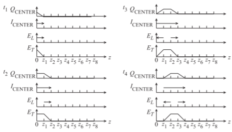
Figure \(\PageIndex{2}\): Fields, currents, and charges on the coaxial transmission line of Figure 2.1.2 at times \(t_{4} > t_{3} > t_{2} > t_{1}\). \(Q_{\text{CENTER}}\) is the net free charge on the center conductor. \(I_{\text{CENTER}}\) is the current on the center conductor.
is denoted \(E_{T}\), and the component directed along the line is denoted \(E_{L}\). (The subscripts \(T\) and \(L\) denote transverse and longitudinal components, respectively.) Thus, while \(E_{L} ≪ E_{T}\), it is necessary to accelerate electrons on the conductors and so give rise to current flow, and hence the movement of the pulse along the line. The electrons do not accelerate indefinitely, as they collide with atoms and scatter so that there is a net velocity of free electrons along the inner and outer conductors.
Snapshots of a pulse traveling along a line are shown in Figure \(\PageIndex{2}\) at four different times.