2.1: Introduction

Filters are the most fundamental of signal processing circuits using energy storage elements to obtain frequency-dependent characteristics. Some of the important filter attributes are (1) controlling noise by not allowing out-of-band noise to propagate in a circuit; (2) keeping signals outside the transmit band, especially harmonics, from being transmitted; and (3) presenting only signals in a specified band to active receive circuitry. At microwave frequencies a filter can consist solely of lumped elements, solely of distributed elements, or a mix of lumped and distributed elements. The distributed realizations can be transmission line-based implementations of the components of lumped-element filter prototypes or, preferably, make use of the particular frequency characteristics found with certain distributed structures. Loss in lumped elements, particularly above a few gigahertz, means that the performance of distributed filters nearly always exceeds that of lumped-element filters. However, since the basic component of a distributed filter is a one-quarter wavelength long transmission line, distributed filters can be prohibitively large below a few gigahertz.

Only a few basic types of responses are required of most RF filters as follows:

1. Lowpass—providing maximum power transfer at frequencies below the corner frequency, \(f_{0}\). Above \(f_{0}\), transmission is blocked. See Figure \(\PageIndex{1}\)(a).
2. Highpass—passing signals at frequencies above \(f_{0}\). Below \(f_{0}\), transmission is blocked. See Figure \(\PageIndex{1}\)(b).
3. Bandpass—passing signals at frequencies between lower and upper corner frequencies (defining the passband) and blocking transmission outside the band. This is the most common type of RF filter. See Figure \(\PageIndex{1}\)(c).
4. Bandstop (or notch)—which blocks signals between lower and upper corner frequencies (defining the stopband). See Figure \(\PageIndex{1}\)(d).
5. Allpass—which equalizes a signal by adjusting the phase generally to correct for phase distortion elsewhere. See Figure \(\PageIndex{1}\)(e).

The above list is not comprehensive, as actual operating conditions may mandate specific frequency profiles. For example, WiFi systems operating at \(2.45\text{ GHz}\) are susceptible to potentially large signals being transmitted from nearby cellular phones operating in the \(1700–2300\text{ MHz}\) range. Thus a frontend filter for a \(2.45\text{ GHz}\) system must ensure very high levels of attenuation over the \(1700–2300\text{ MHz}\) range. Thus the optimum solution here, probably, will have an asymmetrical frequency response with high rejection on one side of the passband obtained by accepting lower rejection on the other side.

2.1.1 Filter Prototypes

In the 1960s an approach to RF filter design and synthesis was developed and this is still followed. The approach is to translate the mathematical response of a lowpass filter. A filter with the desired lowpass response is then synthesized using lumped elements and the resulting filter is called a lowpass prototype. The lowpass filter is then transformed so that the new lumped-element filter has the desired RF response, such as highpass or bandpass. In the case of a bandpass filter, each inductor and capacitor of the lowpass prototype becomes a resonator that is coupled to another resonator. In distributed form, this basic resonator is a one-quarter wavelength long transmission line.

Filter synthesis is a systematic approach to realizing circuits with desired frequency characteristics. A filter can also be thought of as a hardware implementation of a differential equation producing a specific impulse,

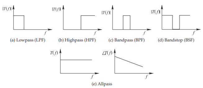
Figure \(\PageIndex{1}\): Ideal filter transfer function, \(T(f)\), responses.

step, or frequency response. It is not surprising that a filter can be described this way as the lumped reactive elements, \(L\) and \(C\), describe first-order differential equations and their interconnection describes higher-order differential equations.

The synthesis of a filter response begins by identifying the desired differential equation response. The differential equations are specified using the Laplace variable, \(s\), so that in the frequency domain (with \(s =\jmath\omega\)) an \(n\)th-order differential equation becomes an \(n\)th-order polynomial expression in \(s\). If possible, and this is usually the case, a lowpass version of a filter can be developed. The conversion to the final filter shape, say a bandpass response, proceeds mathematically through a number of stages. Each stage has a circuit form and each stage is called a filter prototype.

2.1.2 Image Parameter Versus Insertion loss Methods

Filter networks can be synthesized using the image parameter method or the reflection coefficient (or insertion loss) method [1]. The image parameter measured is based on cascading two-port networks with each two-port having the essential desired filter response [2]. Several of these two-ports are cascaded to achieve a periodic-like structure that has the final desired filter response. This method is restrictive and arbitrary filter responses can not be obtained. It is rarely used in RF and microwave filter design but is useful in analyzing simple structures with cascades of identical elements [3]. A better approach is to use the insertion loss method as used in this chapter.