2.2: Singly and Doubly Terminated Networks

Filters are generally two-port networks and they provide maximum power transfer from a source to a load over a specified frequency range while rejecting the transmission of signals at other frequencies. Two possible filter networks are shown in Figure \(\PageIndex{1}\). The network in Figure \(\PageIndex{1}\)(a) is known as a doubly terminated network, as both ports are resistively terminated.

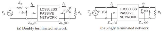
Figure \(\PageIndex{1}\): Terminated networks.

The network in Figure \(\PageIndex{1}\)(b) is called a singly terminated network, as only one port is terminated in a resistor. The doubly terminated network is much closer to the type of network required at RF where loads and source impedances are finite. A singly terminated network is applicable in some RF integrated circuit applications where very little RF power is involved and often when feedback is used. In such cases the output of an RFIC amplifier can approximate an ideal voltage source as the Thevenin equivalent source impedance can be negligible. Most synthesis of singly terminated filter networks uses an analogous procedure to that presented here for doubly terminated filters.

2.2.1 Double Terminated Networks

The established filter synthesis procedure for doubly terminated filter networks focuses on realizing the input reflection coefficient. For a lossless filter the square of the reflection coefficient magnitude is one minus the square of the insertion loss and this is the origin of this method being called the insertion loss method.

The input reflection coefficient of the doubly terminated network in Figure \(\PageIndex{1}\)(a) is

\[\label{eq:1}\Gamma_{1}(s)=\frac{Z_{\text{in, 1}}(s)-R_{S}}{Z_{\text{in, 1}}(s)+R_{S}} \]

where the reference impedance is the source resistance, RS, and s is the Laplace variable. In the passband of a filter the reflection coefficient is approximately zero.

There are several other parameters used in filter design and these will be introduced now. The transducer power ratio (TPR) is defined as

\[\begin{align}\text{TPR}&=\frac{\text{Maximum power available from the source}}{\text{Power absorbed by the load}}\nonumber \\ \label{eq:2}&=\frac{\frac{1}{2}(V_{g}(s)/2)^{2}/R_{S}}{\frac{1}{2}V_{2}^{2}(s)/R_{L}}=\left|\frac{1}{2}\sqrt{\frac{R_{L}}{R_{S}}}\frac{V_{g}(s)}{V_{2}(s)}\right|^{2}\end{align} \]

The transmission coefficient, \(T(s)\), of the network is

\[\label{eq:3}T(s)=\frac{1}{\sqrt{\text{TPR}(s)}}=2\sqrt{\frac{R_{S}}{R_{L}}}\frac{V_{2}(s)}{V_{g}(s)} \]

IF the filter is lossless, the insertion loss (IL) (or transducer function) is

\[\label{eq:4}\text{IL}(s)=\text{TPR}(s)=[1/T(s)]^{2} \]

The next step in development of the filter synthesis procedure is introduction of the characteristic function, defined as the ratio of the reflection and transmission coefficients:

\[\label{eq:5}K(s)=\frac{\Gamma_{1}(s)}{T(s)}=\frac{N(s)}{D(s)} \]

where \(N\) is the numerator function and \(D\) is the denominator function. Ideally the filter network is lossless and so, from the principle of energy conservation, the sum of the magnitudes squared of the transmission and reflection coefficients must be unity:

\[\label{eq:6}|T(s)|^{2}+|\Gamma_{1}(s)|^{2}=1 \]

That is,

\[\label{eq:7}|T(s)|^{2}=1-|\Gamma_{1}(s)|^{2} \]

Dividing both sides of Equation \(\eqref{eq:7}\) by \(|T(s)|^{2}\) results in

\[\label{eq:8}1=\frac{1}{|T(s)|^{2}}-\frac{|\Gamma_{1}(s)|^{2}}{|T(s)|^{2}} \]

or

\[\label{eq:9}1=|\text{IL}(s)|-|K(s)|^{2} \]

Rearranging Equation \(\eqref{eq:9}\) leads to

\[\label{eq:10}|\text{IL}(s)|=1+|K(s)|^{2} \]

and so

\[\label{eq:11}|T(s)|^{2}=\frac{1}{1+|K(s)|^{2}} \]

and

\[\label{eq:12}|\Gamma_{1}(s)|^{2}=\frac{|K(s)|^{2}}{1+|K(s)|^{2}} \]

In the above it is seen that both the reflection and transmission coefficients are functions of the characteristic function of the two-port network. A milestone has been reached. In an RF filter, the frequency-dependent insertion loss or transmission coefficient is of most importance, as these are directly related to power flow. Equation \(\eqref{eq:11}\) shows that this can be expressed in terms of another function, \(K(s)\), which, from Equation \(\eqref{eq:5}\), can be expressed as the ratio of \(N(s)\) and \(D(s)\). For lumped-element circuits, \(N(s)\) and \(D(s)\) are polynomials.

2.2.2 Lowpass Filter Response

As an example of the relationship of the various filter responses, consider the lossless lowpass filter responses shown in Figure \(\PageIndex{1}\). This filter has a lowpass response with a corner frequency expressed in radians as \(\omega_{c} = 1\text{ rad/s}\). Ideally \(T(s)\) for \(s\leq\jmath\) (note \(s =\jmath\omega\)) would be one, and for \(s>\jmath\), \(T(s)\) would be zero. It is not possible to realize such an ideal response, and the response shown in Figure \(\PageIndex{2}\)(a) is typical of what can be achieved. The reflection coefficient is shown in Figure \(\PageIndex{2}\)(b), with the characteristic function \(K(s)\) shown in Figure \(\PageIndex{2}\)(c). If \(|K(s)|^{2}\) is expressed as the ratio of two polynomials (i.e, as \(N(s)/D(s)\)), then it can be seen from Figure \(\PageIndex{2}\)(e and f) that the zeros of the reflection coefficient, \(|\Gamma_{1}(s)|^{2}\), are also the zeros of \(N(s)\). Also, it is observed that the zeros of the transmission coefficient are also the zeros of \(D(s)\), as shown in Figure \(\PageIndex{2}\)(a and c).

The first objective in lumped-element filter design is development of the transfer function of the network in the frequency domain or, equivalently, the \(s\) domain.\(^{1}\) The input-output transfer function of the generic filter in Figure \(\PageIndex{3}\) is

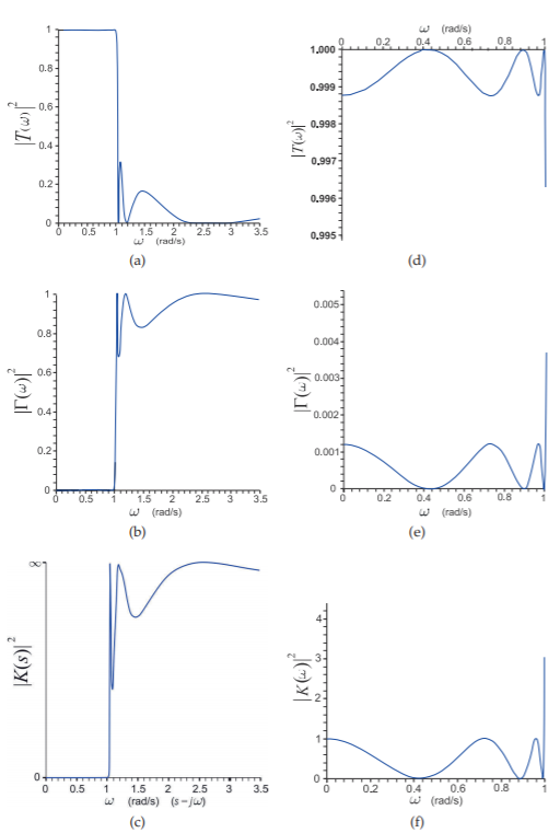
Figure \(\PageIndex{2}\): An example of a lowpass filter in terms of various responses: (a) transmission coefficient; (b) reflection coefficient response; and (c) characteristic function response. Detailed responses are shown in (d), (e), and (f), respectively.

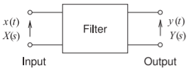
Figure \(\PageIndex{3}\): Generic filter.

\[\label{eq:13}T(s)=Y(s)/X(s) \]

and the design procedure is to match this response to a response defined by the ratio of two polynomials:

\[\label{eq:14}T(s)=\frac{N(s)}{D(s)}=\frac{a_{m}s^{m}+a_{m-1}s^{m-1}+\cdots +a_{1}s+a_{0}}{s^{n}+b_{n-1}s^{n-1}+\cdots +b_{1}s+b_{0}} \]

Here \(N\) stands for numerator and \(D\) for denominator, and these are not the same as those in Equation \(\eqref{eq:5}\) (where they were just labels for numerator and denominator). The filter response using a pole-zero description can be synthesized so the design process begins by rewriting Equation \(\eqref{eq:14}\) explicitly in terms of zeros, \(z_{m}\), and poles, \(p_{n}\):

\[\label{eq:15}T(s)=\frac{N(s)}{D(s)}=\frac{a_{m}(s+z_{1})(s+z_{2})\cdots (s+z_{m-1})(s+z_{m})}{(s+p_{1})(s+p_{2})\cdots (s+p_{n-1})(s+p_{n})} \]

Since only the frequency response is of interest, \(s =\jmath\omega\), thus simplifying the analysis for sinusoidal signals.

The poles and zeros can be complex numbers and can be plotted on the complex \(s\) plane. Conditions imposed by realizable circuits require that \(D(s)\) be a Hurwitz polynomial,\(^{2}\) which ensures that its poles are located in the left-half plane. \(N(s)\) determines the location of the transmission zeros of the filter, and the order of \(N(s)\) cannot be more than the order of \(D(s)\). That is, \(n\geq m\) so that the filter has finite or zero response at infinite frequency

Two strategies can be employed in deriving the filter response. The first is to derive the polynomials \(N(s)\) and \(D(s)\) in Equation \(\eqref{eq:14}\). This seems like an open-ended problem, but it was discovered in the 1950s and 1960s that in normal situations there are only a few types of useful responses that are described by a few polynomials, including Butterworth, Bessel, Chebyshev, and Cauer polynomials.

Footnotes

[1] Care is being taken in the use of terminology as \(s\) can be complex with some filter types, but these filters are realized using digital signal processing.

[2] A Hurwitz polynomial is a polynomial whose coefficients are positive real numbers and whose zeros are located in the left-half of the complex \(s\) plane.