2.4: The Maximally Flat (Butterworth) Lowpass Approximation

Butterworth filters have a maximally flat response (Figure \(\PageIndex{1}\)) that in the time domain corresponds to a critically damped system.

2.4.1 Butterworth Filter Design

Butterworth filters have the transfer function

\[\label{eq:1}T(s)=\frac{N(s)}{D(s)}=\frac{k}{s^{n}+b_{n-1}s^{n-1}+\cdots +b_{1}s+b_{0}} \]

This is an all-pole response. The characteristic polynomial of the Butterworth filter is

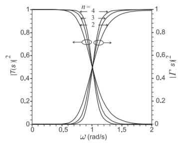
Figure \(\PageIndex{1}\): Maximally flat, or Butterworth, lowpass filter approximation for various orders, \(n\), of the filter.

\(n\)	Factors of \(B_{n}(s)\)
\(1\)	\((s + 1)\)
\(2\)	\((s^{2} + 1.4142s + 1)\)
\(3\)	\((s + 1)(s^{2} + s + 1)\)
\(4\)	\((s^{2} + 0.7654s + 1)(s^{2} + 1.8478s + 1)\)
\(5\)	\((s + 1)(s^{2} + 0.6180s + 1)(s^{2} + 1.6180s + 1)\)
\(6\)	\((s^{2} + 0.5176s + 1)(s^{2} + 1.4142s + 1)(s^{2} + 1.9319s + 1)\)
\(7\)	\((s + 1)(s^{2} + 0.4450s + 1)(s^{2} + 1.2470s + 1)(s^{2} + 1.8019s + 1)\)
\(8\)	\((s^{2} + 0.3902 + 1)(s^{2} + 1.1111s + 1)(s^{2} + 1.6629s + 1)(s^{2} + 1.9616s + 1)\)

Table \(\PageIndex{1}\): Factors of the \(B_{n}(s)\) polynomial.

\[\label{eq:2}|K(s)|^{2}=|s^{2n}|=\omega^{2n} \]

since \(s =\jmath\omega\) and where \(n\) is the order of the function. Thus the transmission coefficient is

\[\label{eq:3}|T(s)|^{2}=\frac{1}{1+|K(s)|^{2}}=\frac{1}{1+|s^{2n}|}=\frac{1}{1+\omega^{2n}} \]

which is often written as

\[\label{eq:4}|T(s)|^{2}=\frac{1}{1+|K(s)|^{2}}=\frac{1}{B_{n}(s)B_{n}(-s)} \]

In the filter community, \(B_{n}(s)\) is called the Butterworth polynomial and has the general form

\[\label{eq:5}B_{n}(s)=\left\{\begin{array}{ll}{\prod_{k=1}^{n/2}\left[s^{2}-2s\cos\left(\frac{2k+n-1}{2n}\pi\right)+1\right]}&{\text{for }n\text{ even}}\\{(s+1)\prod_{k=1}^{(n-1)/2}\left[s^{2}-2s\cos\left(\frac{2k+n-1}{2n}\pi\right)+1\right]}&{\text{for }n\text{ odd}}\end{array}\right. \]

\(B_{n}(s)\) is given in factorized form in Table \(\PageIndex{1}\). Further factorization of the second-order factors results in complex conjugate roots, so they are generally left in the form shown.

Insight is gained by examining the characteristic polynomial for a real radian frequency, \(\omega\) (where \(s =\jmath\omega\)), at the following frequency points:

\[\begin{align}\label{eq:6}\text{at }\omega &=0\quad \to\quad |T(0)|^{2}=\frac{1}{1+0}=1 \\ \label{eq:7}\text{at }\omega&=1\quad\to\quad |T(1)|^{2}=\frac{1}{1+1}=\frac{1}{2}\end{align} \]

Thus the transmission response of the filter is at half power at the corner frequency \(\omega = 1\). Another observation is that the transmission coefficient at \(\omega = 0\) and \(\omega = 1\) are independent of the degree of the characteristic polynomial. This is shown in Figure \(\PageIndex{1}\), where the responses of Butterworth filters are plotted for three different orders.

2.4.2 Construction of the Transfer Function

Often the characteristic function, \(K\), is specified in terms of the variable \(\omega\), and for synthesis purposes the response must be transformed back to the \(s\) domain. As an example, consider the maximally flat function of third order with a characteristic polynomial equal to \(\omega^{3}\) (from Equation \(\eqref{eq:3}\)):

\[\label{eq:8}K(\omega)=\omega^{3}\quad\text{and}\quad |T(\omega)|^{2}=\frac{1}{1+\omega^{6}} \]

(Note that here the first six derivatives of \(|K(s)|^{2}\) with respect to \(s\) are zero at \(s = 0\).) So, from Equation (2.2.7),

\[\label{eq:9}|\Gamma_{1}(\omega)|^{2}=1-\frac{1}{1+\omega^{6}}=\frac{\omega^{6}}{1+\omega^{6}} \]

At real frequencies (i.e., frequencies lying on the imaginary axis in the \(s\) plane)

\[\label{eq:10}s=\jmath\omega,\quad\text{so}\quad\omega=s/\jmath=-\jmath s \]

Thus, in the \(s\) domain, the reflection coefficient becomes

\[\label{eq:11}|\Gamma_{1}(\jmath\omega)|^{2}=|\Gamma_{1}(\jmath(-\jmath s))|^{2}=|\Gamma_{1}(s)|^{2}=\frac{(-\jmath s)^{6}}{1+(-\jmath s)^{6}} \]

That is,

\[\label{eq:12}|\Gamma_{1}(s)|^{2}=\frac{-s^{6}}{1-s^{6}}=\Gamma_{1}(s)\Gamma_{1}(-s) \]

Factoring the denominator polynomial yields

\[\label{eq:13}1-s^{6}=(1-s)(1+s)(s^{2}+s+1)(s^{2}-s+1) \]

By choosing those factors with roots only in the left-half plane (required for a realizable network), the zeros of the denominator are obtained. Now the numerator of \(|\Gamma_{1}(s)|^{2}\) is easily factored, and since this is third order, it only has three reflection zeros at DC. The resulting function is

\[\label{eq:14}\Gamma_{1}(s)=\frac{s^{3}}{(s+1)(s^{2}+s+1)} \]

and so

\[\label{eq:15}T(s)=\frac{1}{(s+1)(s^{2}+s+1)} \]

This example illustrates how \(\Gamma_{1}(s)\) and \(T(s)\) can be obtained from \(K(s)\). This procedure is generalized in the next section.

2.4.3 \(n\)th-Order Reflection Approximation

Following the procedure outlined in the previous section, generalization leads to the \(n\)th-order Butterworth response:

\[\begin{align}|\Gamma_{1}(s)|^{2}&=\Gamma_{1}(s)\cdot\Gamma_{1}(-s)\nonumber \\ \label{eq:16}&=\frac{(-s^{2})^{n}}{1+(-s^{2})^{n}}=\frac{(-s^{2})^{n}}{\prod_{i=1}^{n}(s-s_{i})\cdot\prod_{j=n+1}^{2n}(s-s_{j})}\end{align} \]

So \(|\Gamma_{1}(s)|^{2}\) has \(n\) roots (these are the \(s_{i}\)s) lying in the left-half \(s\) plane, and \(n\) roots (the \(s_{j}\)s) lying in the right-half \(s\) plane. Note that \(j\) is used as an index and \(\jmath\) (\(\jmath\), without the dot) represents \(\sqrt{-1}\). It is reasonable to group all of the left-half plane roots together (a circuit could not be synthesized if there were a right-half plane root) so that

\[\label{eq:17}\Gamma_{1}(s)=\frac{(-s)^{n}}{\prod_{i=1}^{n}(s-s_{i})} \]

Solving for the roots of the denominator of Equation \(\eqref{eq:16}\) (i.e., finding the roots of \(1 +(-s^{2})^{n} = 0\)) yields the following roots in the left-half \(s\) plane:

\[\label{eq:18}s_{i}=\exp\left\{\jmath (2i-1+n)\frac{\pi}{2n}\right\}\quad i=1,2,\ldots ,n \]

where \(\exp (\jmath\theta) = \cos (\theta) + \jmath\sin (\theta)\).

Example \(\PageIndex{1}\): Reflection Coefficient Derivation for Butterworth Filter

Develop the reflection coefficient from the roots of the third-order \((n = 3)\) Butterworth lowpass filter prototype.

Solution

From Equation \(\eqref{eq:18}\) the three roots are

\[\begin{align}\label{eq:19}s_{1}&=\exp\left\{\jmath(2\times 1-1+3)\frac{\pi}{2\times 3}\right\}=\exp\left\{\jmath\frac{2}{3}\pi\right\} \\ \label{eq:20}s_{2}&=\exp\left\{\jmath(2\times 2-1+3)\frac{\pi}{2\times 3}\right\}=\exp\left\{\jmath\:\pi\right\} \\ \label{eq:21}s_{3}&=\exp\left\{\jmath(2\times 3-1+3)\frac{\pi}{2\times 3}\right\}=\exp\left\{\jmath\frac{4}{3}\pi\right\}\end{align} \]

and the input reflection coefficient of the filter normalized to \(1\:\Omega\) is

\[\label{eq:22}\Gamma_{1}(s)=\frac{s^{3}}{\left(s+\frac{1}{2}-\jmath\frac{\sqrt{3}}{2}\right)(s+1)\left(s+\frac{1}{2}+\jmath\frac{\sqrt{3}}{2}\right)}=\frac{s^{3}}{(s+1)(s^{2}+s+1)} \]

This is the same as Equation \(\eqref{eq:14}\).

2.4.4 Bandwidth Consideration

At the corner frequency of the Butterworth response, that is, at \(1\text{ rad/s}\), the transmission response is \(3\text{ dB}\) down from its maximum transfer response.

Order, \(n\)
\(n=3\)	\(4\)	\(5\)	\(6\)	\(7\)	\(8\)	\(9\)	\(10\)
\(0.798\text{ rad/s}\)	\(0.844\)	\(0.873\)	\(0.901\)	\(0.908\)	\(0.919\)	\(0.928\)	\(0.935\)

Table \(\PageIndex{2}\): Radian frequencies at which the response of a Butterworth filter is \(1\text{ dB}\) down for a corner frequency \(f_{0} = 0.1592\text{ Hz}\) (\(\omega_{0} = 1\text{ rad/s}\)). At \(f_{0}\) the transmission response is down \(3\text{ dB}\).

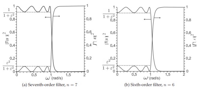
Figure \(\PageIndex{2}\): Chebyshev lowpass filter responses. In decibels, the ripple is \(R_{\text{dB}} = −10 \log[1/(1 + \varepsilon^{2})] = 10 \log(1 + \varepsilon^{2})\), \(\varepsilon\) is called the ripple factor.

Sometimes microwave filters are designed to have \(1\text{ dB}\) bandwidths. The radian frequencies at which the responses of various orders of Butterworth filters are \(1\text{ dB}\) down are given in Table \(\PageIndex{2}\). By frequency scaling the Butterworth response the filter can be design for a specified \(1\text{ dB}\) bandwidth.