2.12: Richards’s Transformation

Richards’s transformation is a remarkable scheme that takes into account the actual properties of transmission lines, yielding broadband transmission line-based implementations of lumped-element filter prototypes [12, 13, 14, 15].

2.12.1 Richard's Transformation and Transmission Lines

Consider a section of transmission line of electrical length \(\theta\) with \(ABCD\) parameters

\[\label{eq:1}T=\left[\begin{array}{cc}{\cos(\theta)}&{\jmath Z_{0}\sin(\theta)}\\{\jmath /Z_{0}\sin(\theta)}&{\cos (\theta)}\end{array}\right] \]

If this line is terminated in a load, \(Z_{L}\), then its input impedance is

\[\label{eq:2}Z_{\text{in}}(\theta)=\frac{\cos(\theta)Z_{L}+\jmath Z_{0}\sin(\theta)}{\jmath /Z_{0}\sin(\theta)Z_{L}+\cos(\theta)} \]

Now examine two extreme conditions. As the load impedance increases, eventually becoming an open circuit, the input impedance of a line with electrical length \(\theta\) is defined in terms of a cotangent of the electrical length:

\[\begin{align}\label{eq:3}Z_{L}\to\infty\quad \Rightarrow Z_{\text{in}}(\theta)&=\frac{Z_{0}}{\jmath}\cot(\theta) \\ \label{eq:4}Y_{\text{in}}(\theta)&=\jmath Y_{0}\tan(\theta)\end{align} \]

As the load impedance reduces to become a short circuit, the input impedance of a line with electrical length \(\theta\) is defined in terms of a tangent of the electrical length:

\[\label{eq:5}Z_{L}\to 0\quad\Rightarrow\quad Z_{\text{in}}(\theta)=\jmath Z_{0}\tan(\theta) \]

These results lead to the Richards’s transformation, which replaces the Laplace variable, \(s\), by Richards’s variable, \(S\), where \(S =\jmath\alpha\tan(\theta)\). This transformation is written

\[\label{eq:6}s\to S=\jmath\alpha\tan(\theta) \]

For now \(\alpha\) and \(\theta\) are constants that can be chosen as design variables. \(\theta\), of course, is the electrical length of the line. Also, \(\alpha\) must have the units of impedance and it is the characteristic impedance of the transmission line.

Applying the Richards’s transformation to a capacitor, the admittance of the element is transformed as follows:

\[\label{eq:7}y=sC\to Y=SC=\jmath\alpha C\tan(\theta) \]

so that the capacitor is transformed into an open-circuited stub with characteristic admittance

\[\label{eq:8}Y_{0}=\alpha C \]

If a lumped-element capacitor with admittance \(y = sC\) is to be realized using a transmission line, the admittance \(Y = SC =\jmath\alpha C \tan(\theta )\) is instead realized. There are two parameters to select to realize this admittance. The first, \(\alpha\), is the characteristic admittance of the transmission line (and for any given transmission line topology there is a minimum and maximum characteristic admittance or impedance that can be realized), and \(\theta\) is the electrical length of the line.

Applying the transformation to an inductor, the impedance of the element is transformed as follows:

\[\label{eq:9}Z=sL\to Z=SL=\jmath\alpha L\tan(\theta) \]

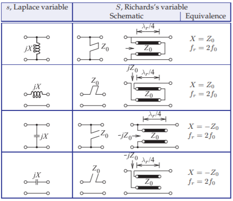
Figure \(\PageIndex{1}\): Equivalences resulting from Richards’s transformation. With \(f_{r} = 2f_{0}\) the transmission line stubs are one-eighth wavelength long at \(f_{0}\).

so that the inductor is transformed into a short-circuited stub with characteristic impedance

\[\label{eq:10}Z_{0}=\alpha L \]

Thus the Richards’s transform converts an inductor into a short-circuited stub and a capacitor into an open-circuited stub.

2.12.2 Richard's Transformation and Stubs

There is a duality between stubs and inductors and capacitors; they are coupled by Richards’s transformation. One of the important quantities used in the transformation is the commensurate frequency, \(f_{r}\), which most often is chosen as twice the operating frequency, \(f_{0}\). Considering stubs that are one-quarter wavelength long at \(f_{r}\), the duality is as shown in Figure \(\PageIndex{1}\).

2.13.3 Richard's Transformation Applied to a Lowpass Filter

In this section, Richards’s transformation is used to realize a lumped-element filter in distributed form. The design example begins by considering a Chebyshev lowpass filter with the transmission characteristic

\[\label{eq:11}|T(s)|^{2}=\frac{1}{1+\varepsilon^{2}|K(s)|^{2}} \]

With the Richards’s transformation \((s\to\jmath\omega\to\jmath\alpha\tan (\theta))\) this becomes

\[\label{eq:12}|T(\jmath\alpha\tan\theta)|^{2}=\frac{1}{1+\varepsilon^{2}|K(\jmath\alpha\tan\theta))|^{2}} \]

Thus the passband edge at \(\omega = 1\) is mapped to \(\omega =\theta_{1}\) as

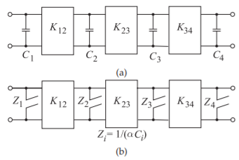
Figure \(\PageIndex{2}\): Lowpass prototypes: (a) lowpass prototype as a ladder filter with inverters; and (b) lowpass distributed prototype with open-circuited stubs (the impedance looking into the stub is indicated).

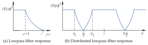
Figure \(\PageIndex{3}\): Lowpass to distributed lowpass transformation. \(s =\jmath\omega\).

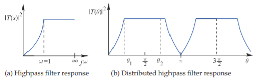
Figure \(\PageIndex{4}\): Highpass to distributed highpass transformation. \(s =\jmath\omega\).

\[\label{eq:13}\omega =1\to\alpha\tan (\theta_{1}) \]

so that

\[\label{eq:14}\alpha=\frac{1}{\tan(\theta_{1})} \]

Recalling that a capacitor is transformed into an open-circuited stub (see Equation \(\eqref{eq:8}\)), Richards’s transformation applied to the lowpass filter prototype results in a filter with transmission line elements only, as shown Figure \(\PageIndex{2}\), provided that the inverters are realized using transmission lines.

The implementation of a lowpass filter in distributed form results in passbands and stopbands that repeat in frequency, as shown in Figure \(\PageIndex{3}\). This occurs because transmission lines are used to realize lumped elements and the two-port parameters of a transmission line repeat every wavelength (or one-half wavelength in some cases). For example, the input impedance of a stub is the same whether it is one-half wavelength long or one wavelength long.

2.12.4 Richard's Transformation Applied to a Highpass Filter

With reference to Figure \(\PageIndex{4}\)(a), the passband edge at \(\omega = 1\) is mapped to \(\theta_{1}\), as shown in Figure \(\PageIndex{4}\)(b). This means that the passband at \(\omega = 1\) is mapped

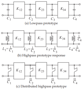
Figure \(\PageIndex{5}\): Ladder prototype transformation. (The input impedances of the stubs are indicated in (c).)

to \(\theta_{1}\) as (note that \(\theta_{1}\) is the electrical length at the band edge)

\[\label{eq:15}\omega =1\to\alpha\tan(\theta_{1}) \]

so that

\[\label{eq:16}\alpha =\frac{1}{\tan(\theta_{1})} \]

The sequence of steps transforming a lumped lowpass prototype to its distributed highpass prototype are shown in Figure \(\PageIndex{5}\). As previously discussed, all the inverters can be approximated by transmission lines of length \(\pi /2\) at the corner frequency of the filter.