4.4: Noise Characterization

Amplifiers, filters, and mixers in an RF front end process (e.g., amplify, filter, and mix) input noise the same way as an input signal. In addition, these components contribute excess noise of their own. Without loss of generality, the following discussion considers noise with respect to the amplifier shown in Figure 4.2.4(a), where \(v_{s}\) is the input signal. The development here applies only to white noise (i.e., thermal and shot noise). The noise signal, with source designated by \(v_{n}\), is uncorrelated and random, and described as an RMS voltage or by its noise power.

The most important noise-related metric is the SNR. Denoting the noise power input to the amplifier as \(N_{i}\), and denoting the signal power input to the amplifier as \(S_{i}\), the input signal-to-noise power ratio is \(\text{SNR}_{i} = S_{i}/N_{i}\). If the amplifier is noise free, then the input noise and signal powers are amplified by the power gain of the amplifier, \(G\). Thus the output noise power is \(N_{o} = GN_{i}\), the output signal power is \(S_{o} = GS_{i}\), and the output SNR is \(\text{SNR}_{o} = S_{o}/N_{o} = \text{SNR}_{i}\).

In practice, an amplifier is noisy, with the addition of excess noise, \(N_{e}\), indicated in Figure 4.2.4(b). The excess noise originates in different components in the amplifier and is either referenced to the input or to the output of the amplifier. Most commonly it is referenced to the output so that the total output noise power is \(N_{o} = GN_{i} + N_{e}\). In the absence of a qualifier, the excess noise should be assumed to be referred to the output. \(N_{e}\) is not measured directly. Instead, the ratio of the SNR at the input to that at the output is the noise factor:

\[\label{eq:1}F=\frac{\text{SNR}_{i}}{\text{SNR}_{o}} \]

and this is the way noise performance is normally measured. If the circuit is noise free, then \(\text{SNR}_{o} = \text{SNR}_{i}\) and \(F = 1\). If the circuit is not noise free, then \(\text{SNR}_{o} < \text{SNR}_{i}\) and \(F > 1\). \(F\) can be related to the excess noise produced in the circuit. With the excess noise, \(N_{e}\), referred to the circuit output,

\[\begin{align}F&=\frac{\text{SNR}_{i}}{\text{SNR}_{o}}=\frac{\text{SNR}_{i}}{1}\frac{1}{\text{SNR}_{o}}=\frac{S_{i}}{N_{i}}\frac{N_{o}}{S_{o}}=\frac{S_{i}}{N_{i}}\frac{GN_{i}+N_{e}}{GS_{i}}\nonumber \\ \label{eq:2}&=1+\frac{N_{e}}{GN_{i}}\end{align} \]

One of the conclusions that can be drawn from this is that the noise factor, \(F\), depends on the available noise power at the input of the circuit. As a standard reference, the available noise power, \(N_{R}\), from a resistor at standard temperature, \(T_{0}\) \((290\text{ K})\) [12], and over a bandwidth, \(B\) (in \(\text{Hz}\)), is used,

\[\label{eq:3}N_{i}=N_{R}=kT_{0}B \]

where \(k (= 1.381\times 10^{−23}\text{ J/K})\) is the Boltzmann constant. If the input of an amplifier is connected to this resistor and all of the noise power is delivered to the amplifier, then

\[\label{eq:4}F=1+\frac{N_{e}}{GN_{i}}=1+\frac{N_{e}}{GkT_{0}B} \]

Several random physical processes inside a circuit contribute to excess noise, and not all of these processes vary linearly with temperature. Consequently \(F\) is a function of temperature, although usually a weak one. It is also a function of bandwidth, and there is a problem in using \(F\) with cascaded systems in which bandwidths vary for different subsystems. Even with all these problems, \(F\) is the most important measure used to characterize noise performance. It can be used to determine the noise performance of a cascade, when the noise factors and gains of the subsystem constituents are known. \(F\) is the ratio of powers, and when expressed in decibels, the noise figure (NF) is used:

\[\begin{align}\text{NF}&=10\log_{10}F\nonumber \\ \label{eq:5}&=\text{SNR}_{i}|_{\text{dB}}-\text{SNR}_{o}|_{\text{dB}}\end{align} \]

where the SNR is expressed in decibels.

Consider the amplifier in Figure 4.2.4. If the excess noise contribution of an amplifier is ignored, the output noise power will be

\[\label{eq:6}N_{o}=GkT_{0}B \]

With the amplifier’s excess noise, \(N_{e}\), included, the output noise power is

\[\begin{align}N_{o}&=GkT_{0}B+N_{e}=GkT_{0}B(1+N_{e}/(GkT_{0}B))\nonumber \\ \label{eq:7}&=FGkT_{0}B\end{align} \]

Rearranging this equation, the excess noise power can be written as

\[\label{eq:8}N_{e}=(F-1)GkT_{0}B \]

The output noise of a system can be expressed in terms of its noise figure. From Equation \(\eqref{eq:4}\), the output noise is

\[\label{eq:9}N_{o}=GN_{i}+N_{e}=FGN_{i} \]

That is,

\[\label{eq:10}N_{o}|_{\text{dBM}}=\text{NF}+G|_{\text{dB}}+N_{i}|_{\text{dBM}} \]

So if the input noise of an amplifier with a gain of \(20\text{ dB}\) and a noise figure of \(3\text{ dB}\) is \(−90\text{ dBm}\), then the noise at the output of the amplifier is \(−67\text{ dBm}\). This analysis of output noise is only correct if the input source is the equivalent of a resistor held at standard temperature, \(T_{0}\). So the analysis would not apply if the input to the system was an antenna pointed into the sky (away from cosmic objects such as the sun and moon) which would have a noise temperature of \(4\text{ K}\) (due to the cosmic background radiation) plus antenna and cable noise.

Example \(\PageIndex{1}\): Effective Noise Temperature

An antenna with a noise temperature of \(50\text{ K}\) is connected to an amplifier with a bandwidth of \(20\text{ MHz}\), a noise figure of \(3\text{ dB}\), and a gain of \(10\text{ dB}\). What is the effective noise temperature at the output of the amplifier?

Solution

The output effective noise temperature, \(T_{\text{eff}}\), is the temperature of a resistor that would produce the same available noise power, \(N_{o}\), as the output available noise power of the amplifier. The amplifier adds excess noise, \(N_{e}\), to the input noise, \(N_{i}\), that is amplified by the amplifier. So to determine \(N_{o}\), \(N_{e}\) must be determined first. This is obtained from the noise figure, \(\text{NF}\), which is defined in terms of noise power of a resistor at the input with a temperature of \(T_{0} = 290\text{ K}\).

The noise factor \(F = 10^{\text{NF}} = 1.995\) and from Equation \(\eqref{eq:8}\)

\[\begin{align}N_{e}&= (F − 1)GkT_{0}B = (1.995 − 1)\cdot 10^{10/10}\cdot (1.3807\cdot ^{−23}\text{ J/K})\cdot (290\text{ K})\cdot (20\cdot 10^{6}\text{ Hz})\nonumber \\ \label{eq:11} &=7.969\cdot 10^{-13}\text{ W}\end{align} \]

The input noise of a resistor at \(50\text{ K}\) is

\[\label{eq:12}N_{i}=kTB= (1.3807\cdot^{−23}\text{ J/K})\cdot (50\text{ K})\cdot (20\cdot 10^{6}\text{ Hz}) = 1.381\cdot 10^{−14}\text{ W} \]

So the total output noise power is

\[\label{eq:13}N_{o} = GN_{i} + N_{e} = 10^{10/10}\cdot 1.381\cdot 10^{−14} + 7.969\cdot 10^{−13} = 9.350\cdot 10^{−13}\text{ W} \]

Thus the effective noise temperature at the output of the amplifier is

\[\label{eq:14}T_{\text{eff}}=\frac{N_{o}}{kB}=\frac{9.350\cdot 10^{-13}\text{ W}}{(1.3807\cdot ^{−23}\text{ J/K})\cdot (20\cdot 10^{6}\text{ Hz})}=3386\text{ K} \]

Example \(\PageIndex{2}\): Noise Figure of an Attenuator

What is the noise figure of a \(20\text{ dB}\) attenuator in a \(50\:\Omega\) system?

Solution

Denoting the attenuator as being in a \(50\:\Omega\) system indicates that an appropriate circuit model to use in the analysis consists of the attenuator driven by a generator with a \(50\:\Omega\) source impedance, and the attenuator drives a \(50\:\Omega\) load. Also, the input impedance of the terminated attenuator is \(50\:\Omega\), as is the impedance looking into the output of the attenuator when it is connected to the source. The key point is that the noise coming from the source is the noise thermally generated in the \(50\:\Omega\) source impedance, and this noise is equal to the noise that is delivered to the load, as the impedance presented to the load is also \(50\:\Omega\). So the input noise, \(N_{i}\), is equal to the output noise:

\[\label{eq:15}N_{o}=N_{i} \]

The input signal is attenuated by \(20\text{ dB} (= 100)\), so

\[\label{eq:16}S_{o}=S_{i}/100 \]

and thus the noise factor is

\[\label{eq:17}F=\frac{SNR_{i}}{SNR_{o}}=\frac{S_{i}}{N_{i}}\frac{N_{o}}{S_{o}}=\frac{S_{i}}{N_{i}}\frac{N_{i}}{S_{i}/100}=100 \]

and the noise figure is

\[\label{eq:18}\text{NF}=20\text{ dB} \]

Thus the noise figure of an attenuator (or a filter) is just the loss of the component. This is not true for amplifiers of course, as there are other sources of noise, and the output impedance of a transistor is not a thermal resistance.

4.3.1 Noise in a Cascaded System

Section 4.3 developed the noise factor and noise figure measures for a two-port. This result can be generalized for a system. Considering the second stage of the cascade in Figure \(\PageIndex{1}\), the excess noise at the output of the second stage, due solely to the noise generated internally in the second stage, is

\[\label{eq:19}N_{2e}=(F_{2}-1)kT_{0}BG_{2} \]

Then the total noise power at the output of a two-stage cascade is

\[\begin{align}N_{2o}&=(F_{2}-1)kT_{0}BG_{2}+N_{o,1}G_{2}\nonumber \\ \label{eq:20} &=(F_{2}-1)kT_{0}BG_{2}+F_{1}kT_{0}BG_{1}G_{2}\end{align} \]

This relies on the reasonable assumption that the excess noise added in one stage is uncorrelated to the excess noise from other stages as well as being uncorrelated to the input noise. Thus powers can be added. The second term

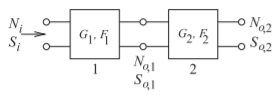
Figure \(\PageIndex{1}\): Cascaded noisy two-ports.

in Equation \(\eqref{eq:20}\) is the noise output from the first stage amplified by the second stage with gain \(G_{2}\).

Generalizing the above result yields the total noise power at the output of the \(m\)th stage:

\[\label{eq:21}N_{mo}=\sum_{n=2}^{m}\left[(F_{n}-1)kT_{0}B\prod_{j=2}^{n}G_{j}\right]+F_{1}kT_{0}B\prod_{n=1}^{m}G_{n} \]

Thus an m-stage cascade has a total cascaded system noise factor of \(F^{T} =N_{mo}/(G^{T}N_{1i}0\), with \(G^{T}\) being the total cascaded available gain and \(N_{1i}\) being the noise power input to the first stage. In terms of the parameters of individual stages, the total system noise factor is

\[\label{eq:22}F^{T}=F_{1}+\frac{F_{2}-1}{G_{1}}+\frac{F_{3}-1}{G_{1}G_{2}}+\frac{F_{4}-1}{G_{1}G_{2}G_{3}}+\ldots \]

that is,

\[\label{eq:23}F^{T}=F_{1}+\sum_{n=2}^{m}\frac{F_{n}-1}{\prod_{i=2}^{n}G_{i-1}} \]

This equation is known as Friis’s formula [13].

Note

The similarly named Friis transmission formula refers to antenna systems.

Example \(\PageIndex{3}\): Noise Figure of Cascaded Stages

Consider the cascade of a differential amplifier and a filter shown in Figure \(\PageIndex{2}\).

1. What is the midband gain of the filter in decibels? Note that IL is insertion loss.
2. What is the midband noise figure of the filter?
3. The amplifier has a gain \(G_{1} = 20\text{ dB}\) and a noise figure of \(2\text{ dB}\). What is the overall gain of the cascade system in the middle of the band? Express your answer in decibels.
4. What is the noise factor of the cascade system?
5. What is the noise figure of the cascade system?

Solution

1. \(G_{2} = 1/\text{IL}\), thus \(G_{2} = −3\text{ dB}\).
2. For a passive element, \(\text{NF}_{2} = \text{IL} = 3\text{ dB}\).
3. \(G_{1} = 20\text{ dB}\) and \(G_{2} = −3\text{ dB}\), so \(G_{\text{TOTAL}} = G_{1}|_{\text{dB}} + G_{2}|_{\text{dB}} = 17\text{ dB}\).
4. \(F_{1} = 10^{\text{NF}_{1}/10} = 10^{2/10} = 1.585,\: F_{2} = 10^{\text{NF}_{2}/10} = 10^{3/10} = 1.995,\: G_{1} = 10^{20/10} = 100,\) and \(G_{2} = 10^{−3/10} = 0.5\). Using Friis’s formula
   \[\label{eq:24}F_{\text{TOTAL}}=F_{1}+\frac{F_{2}-1}{G_{1}}=1.585+\frac{1.995-1}{100}=1.594 \]
5. \(\text{NF}_{\text{TOTAL}}=10\log_{10}(\text{F}_{\text{TOTAL}})=10\log_{10}(1.594)=2.03\text{ dB}\)

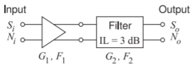
Figure \(\PageIndex{2}\): Differential amplifier followed by a differential filter.

Example \(\PageIndex{4}\): Noise Figure of a Two-Stage Amplifier

Consider a room-temperature \((20^{\circ}\text{C})\) two-stage amplifier where the first stage has a gain of \(10\text{ dB}\) and the second stage has a gain of \(20\text{ dB}\). The noise figure of the first stage is \(3\text{ dB}\) and the second stage is \(6\text{ dB}\). The amplifier has a bandwidth of \(10\text{ MHz}\).

1. What is the noise power presented to the amplifier in \(10\text{ MHz}\)?
2. What is the total gain of the amplifier?
3. What is the total noise factor of the amplifier?
4. What is the total noise figure of the amplifier?
5. What is the noise power at the output of the amplifier in \(10\text{ MHz}\)?

Solution

1. Noise power of a resistor at room temperature is \(−174\text{ dBm/Hz}\) (or more precisely \(−173.86\text{ dBm/Hz}\) at \(293\text{ K}\)). In \(10\text{ MHz}\) the input noise power is \(N_{i} = −173.86\text{ dBm} + 10 \log(10^{7}) = −173.86 + 70\text{ dBm} = −103.86\text{ dBm}\).
2. Total gain \(G^{T} = G_{1}G_{2} = 10\text{ dB} + 20\text{ dB} = 30\text{ dB} = 1000\).
3. \(F_{1} = 10^{\text{NF}_{1}/10} = 10^{3/10} = 1.995,\: F_{2} = 10^{\text{NF}_{2}/10} = 10^{6/10} = 3.981\). Using Friis’s formula, the total noise figure is \(F^{T}= F_{1} + \frac{F_{2} − 1}{G_{1}} = 1.995 + \frac{3.981 − 1}{10} = 2.393\).
4. The total noise figure is \(\text{NF}^{\text{T}} = 10 \log_{10}(F^{T}) = 10 \log_{10}(2.393) = 3.79\text{ dB}\).
5. Output noise power in \(10\text{ MHz}\) bandwidth is \(N_{o} = F^{T}kT_{0}BG^{T} = (2.393)\cdot (1.3807\cdot 10^{−23}\cdot\text{J}\cdot\text{K}^{−1})\cdot (293\text{ K})\cdot (10^{7}\cdot\text{s}^{−1})(1000) = 9.846\cdot 10^{−11}\text{ W} = −70.07\text{ dBm}\). Alternatively, \(N_{o}|_{\text{dBm}} = N_{i}|_{\text{dBm}} + G^{T}|_{\text{dB}} + \text{NF}^{\text{T}} = −103.86\text{ dBm} + 30\text{ dB} + 3.79\text{ dB} = −70.07\text{ dBm}\).

4.3.2 Measurement of Noise Figure

The \(Y\)-factor method is the basis of modern microwave automatic noise figure measurement systems. The technique involves measuring the noise power at the output of a device under test (DUT) when two different noise sources are attached to the input of the DUT [14]. The manual form of the \(Y\)-factor method is used at millimeter-wave frequencies. The method is dependent on the accuracy of gain measurement, the ability to generate precise levels of excess noise power, and the sensitivity of noise power measurement. Gain and noise power measurement are subtly different, with gain generally a coherent measurement while the noise power measurement is necessarily incoherent. In both automatic and manual systems, the measurement setup is a cascade system in which the DUT is the first stage and the test set is the last and usually second set. The noise contribution of the test set is only negligible if the gain of the DUT is high.

Under matched conditions, the available power gain of the DUT is

\[\label{eq:25}G=\frac{S_{o}}{S_{i}} \]

so signal power can be eliminated from the expression for the noise factor by combining Equations \(\eqref{eq:1}\) and \(\eqref{eq:25}\):

\[\label{eq:26}F=\frac{\text{SNR}_{i}}{\text{SNR}_{o}}=\frac{S_{i}}{N_{i}}\frac{N_{o}}{S_{o}}=\frac{N_{o}}{N_{i}G} \]

The output noise is larger than the amplified input noise because of the noise inserted by the DUT. Denoting the component of the output noise power due

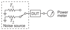
Figure \(\PageIndex{3}\): Noise figure test setup for determining the noise figure of a DUT.

solely to the DUT by \(N_{D}\), the output noise power is

\[\label{eq:27}N_{o}=N_{i}G+N_{D} \]

The final component of the development is noting that the input noise power is related to the temperature of the input match so that \(N_{i} = kTB\) where \(k\) is the Boltzmann constant and \(B\) is the measurement bandwidth. Conventionally \(F\) is referenced to standard temperature \(T_{0} = 290\text{ K}\) (specifically the input noise temperature is \(T_{0}\)) and so

\[\label{eq:28}N_{D}=kT_{0}BG(F-1) \]

In the \(Y\)-factor method, two noise sources with known noise temperatures \(T_{1}\) and \(T_{2}\) (with \(T_{2} > T_{1}\)) are applied to the input of the DUT and the corresponding output noise powers \(N_{1}\) and \(N_{2}\) measured (see Figure \(\PageIndex{3}\)). In the laboratory a calibrated noise source, such as a reverse-biased diode in avalanche, is used to produce the noise source at \(T_{2}\). The other temperature, \(T_{1}\), is often obtained by turning the noise source off so that \(T_{1} = T_{0}\), the ambient temperature. This leads to the \(Y\) factor, which is defined as

\[\label{eq:29}Y=N_{2}/N_{1} \]

In the off state, that is when \(T_{1} = T_{0}\), the output noise power in the off state is called the “off power”:

\[\label{eq:30}N_{1}=kT_{0}BG+N_{D}=kT_{0}BG+kT_{0}BG(F-1) \]

The second noise source, with noise temperature \(T_{2}\), produces calibrated excess noise and the noise power under these conditions is called the “on power”:

\[\label{eq:31}N_{2}=kT_{2}BG+N_{D}=kT_{2}BG+kT_{0}BG(F-1) \]

Combining Equations \(\eqref{eq:28}\)–\(\eqref{eq:31}\) yields

\[\label{eq:32}F=\frac{T_{2}-T_{0}}{T_{0}(Y-1)} \]

Expressing Equation \(\eqref{eq:33}\) in decibels and integrating (perhaps through measurement) over the system bandwidth yields the noise figure,

\[\label{eq:33}\text{NF}=10\log(F)=\text{ENR}_{\text{dB}}-10\log(Y-1) \]

where \(\text{ENR}_{\text{dB}} = 10 \log[(T_{2} − T_{0})/T_{0}]\) is the excess noise ratio in decibels of the calibrated noise source.

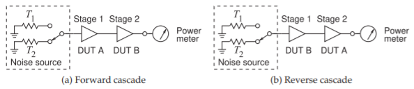
Figure \(\PageIndex{4}\): \(Y\)-factor test set actively incorporating the second-stage contribution effect.

4.3.3 Measurement of Noise Temperature

If the noise figure of an amplifier replacing the DUT is known, then the noise temperature of a source can be determined. From Equation \(\eqref{eq:32}\),

\[\label{eq:34}T_{2}=FT_{0}(Y-1)+T_{0} \]

In a laboratory application the amplifier could be cryogenically cooled and then there is negligible excess noise contribution by the amplifier so that \(F\approx 1\) and \(T_{2} = YT_{0}F\).

4.3.4 Measuring the Noise Figure of Low Noise Devices

One of the factors that affects the accuracy of noise figure determination is noise originating in the measurement test set. This leads to an error sometimes referred to as the second-stage contribution effect [15]. This is a particularly important issue when measuring the noise figure of low-gain devices, as then the noise contribution of the second stage can be significant. One approach to minimizing this error is the insertion of a high-gain lownoise amplifier, referred to as the instrumentation amplifier, between the DUT and the test set. The noise figure of the instrumentation amplifier should be known precisely if the error it introduces is to be removed from the raw noise figure measurement.

The \(Y\)-factor method relies on the instrumentation amplifier having a much lower noise figure than the DUT. When this cannot be achieved, the best that can be done is to use two (almost) identical amplifiers with the same gain and noise characteristics. The extended \(Y\)-factor technique described in this section utilizes two DUTs in a two-stage cascade first with one arrangement of the DUTs and then with the reverse cascade [16]. The technique makes use of the cascaded noise factor operation twice. Figure \(\PageIndex{4}\) illustrates the test setup with the two possible arrangements of the cascaded DUTs. In Figure \(\PageIndex{4}\) the power meter is configured to measure noise power (normalized to a \(1\text{ Hz}\) bandwidth).

The individual noise factors of the DUTs for a cascaded system with DUT A followed by DUT B, the forward cascade, are denoted by \(F_{1A}\) and \(F_{2B}\), and those for the reverse cascade with DUT B followed by DUT A are \(F_{1B}\) and \(F_{2A}\). The corresponding gains of the stages are \(G_{1A},\: G_{2B}\) for the forward cascade, and \(G_{1B},\: G_{2A}\) for the reverse cascade. Here the first subscript refers to the position in the cascade (either first or second stage), and the second subscript identifies the particular DUT (either A or B). Finally, the total noise factors of the two-cascaded systems are denoted \(F_{A}^{T}\) and \(F_{B}^{T}\) according to

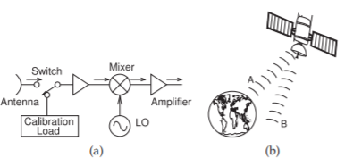
Figure \(\PageIndex{5}\): Radiometer: (a) heterodyne architecture showing calibration switch; and (b) satellite radiometer that switches between two beams, one oriented at the region being monitored and the other at much colder space that serves as calibration.

whether DUT A or DUT B is the first stage. Using Friis’s formula for the forward cascade, Equation \(\eqref{eq:23}\) can be written as,

\[\label{eq:35}F_{A}^{T}=F_{1A}+(F_{2B}-1)/G_{1A} \]

and for the reverse cascade

\[\label{eq:36}F_{B}^{T}=F_{1B}+(F_{2A}-1)/G_{1B} \]

The technique presumes that the parameters of the DUTs are invariant of their position in the cascade so that \(F_{1A} = F_{2A} = F_{A}\) and \(F_{1B} = F_{2B} = F_{B}\) as well as \(G_{1A} = G_{2A} = G_{A}\) and \(G_{1B} = G_{2B} = G_{B}\). Equations \(\eqref{eq:35}\) and \(\eqref{eq:36}\) can now be solved simultaneously for the unknown noise factors of the two stages:

\[\label{eq:37}F_{B} =[F_{B}^{T}G_{A}G_{B}-G_{A}(1 − F_{A}^{T}) − 1]/(G_{A}G_{B}) \]

and

\[\label{eq:38}F_{A}=[F_{A}^{T}G_{A}-F_{B}+1]/(G_{A}) \]

from the measured \(F_{A}^{T},\: F_{B}^{T},\: G_{A}\), and \(G_{B}\). So with the gains of the two stages measured independently, the noise factors of the two stages can be determined from the measured noise factors of the forward and reverse cascades.

In the special situation of matched DUTs where the noise and gain of the two stages are identical (so that \(F_{A} = F_{B} = F\) and \(G_{A} = G_{B} = F\)) and \(F_{A}^{T}= F_{B}^{T}= F^{T}\), then the calculations simplify to yield the noise factor of each stage:

\[\label{eq:39}F=\frac{GF^{T}}{G^{2}+1} \]

One of the assumptions of the extended Y -factor method is that the gain and noise of the stages are invariant with respect to the order of the stages in the cascade. Any departure will result in an error. A technique that reduces the sensitivity to placement is to use small attenuators at the inputs and outputs of the stages. The noise contributions can then be removed from the final measured result.

4.3.5 Radiometer System

A radiometer, as shown in Figure \(\PageIndex{5}\)(a), measures the power in EM radiation predominantly at microwave frequencies and most commonly measures noise. Radiometers are used in remote sensing and radio astronomy,

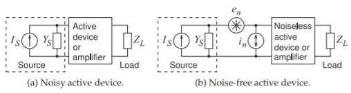
Figure \(\PageIndex{6}\): Amplifier model for noise factor calculation: (a) with noisy active device or amplifier where \(I_{S}\) is the source generator and \(Y_{S}\) is the Norton equivalent admittance of the source; and (b) with the noisy active device or amplifier replaced by the noise voltage, \(e_{n}\), and noise current, \(i_{n}\), (the noise sources), and a lossless active device or amplifier.

especially by satellites and aircraft. Understanding the physical process that creates uncorrelated radiation at different frequencies enables vegetation, air and sea temperatures, ice coverage, ocean salinity, and other surface and atmospheric sources to be identified from the spectrum captured by a radiometer. Radiometers monitor discrete windows of the spectrum, particularly at frequencies corresponding to molecular resonances. A radiometer includes a mechanism for rapid calibration, such as a Dicke switch, quickly switching between the object being observed and another object serving as a calibrated noise source. In aircraft and on land, the calibration sources are resistors, often held at low temperatures. A satellite-based radiometer is shown in Figure \(\PageIndex{5}\)(b), and instead of a Dicke switch, the calibration is obtained by switching the antenna beam between the observed region (Beam A) and an empty area of space (Beam B). With a Dicke switch or antenna beam switching, it is possible to achieve better than 0.01 K of resolution.

4.3.6 Noise Figure of a Two-Port Amplifier

The parameters that define the noise figure of two-port amplifiers were set forth by Haus et al. [12] in 1960 and are used by microwave transistor manufacturers in their datasheets. The amplifier model used in noise factor computation is shown in Figure \(\PageIndex{6}\).

Figure \(\PageIndex{6}\) has the active device or amplifier, which is noisy, represented as a two-port with a Norton equivalent source, which will have its own noise, and a load. The noisy active device or amplifier can be replaced by a noiseless two-port with a voltage noise source, \(e_{n}\), and a current noise source, \(i_{n}\), at the front of the two-port. Any linear noisy two-port can be represented by a noise free two-port with noise sources. With an active device or amplifier there will be many internal noise sources but it is the noise sources at the input, prior to gain, which are most significant. For an active device or amplifier the voltage and current sources will be at least partially correlated and so the source admittance is important in determining how they combine. A worst case would be when they combine to present the maximum possible noise at the input of the active device or amplifier. It is also possible to adjust the source admittance so that the noise sources combine to present the minimum noise to the active device or amplifier. This effect is captured in the noise factor of the amplifier in Figure \(\PageIndex{6}\). The noise factor of this amplifier is [12]

\[\label{eq:40}F=F_{\text{min}}+\frac{r_{n}}{g_{s}}\left| y_{s}-y_{\text{opt}}\right|^{2} \]

where \(r_{n} = (R_{n}/Z_{0})\) is called the equivalent noise resistance of the two-port and \(F_{\text{min}}\) is the minimum noise factor obtained by adjusting tuners at the input of the amplifier to present all possible values of \(Y_{S}\) to the input of the amplifier. The normalized admittance presented by the tuners at \(F_{\text{min}}\) is \(y_{\text{opt}}\). With \(y_{s}(= Y_{S} /Z_{0})\) and \(g_{s} = \Re \{y_{s}\}\) being the actual normalized admittance and conductance, respectively, Equation \(\eqref{eq:40}\) enables the noise factor to be calculated for an actual design. The parameters in Equation \(\eqref{eq:40}\) describe the effect of internal amplifier noise sources and how they are correlated.

More commonly the noise parameters are reported in terms of reflection coefficients rather than admittance. The source reflection coefficient, \(\Gamma_{s}\), comes from

\[\label{eq:41}y_{s}=\frac{1-\Gamma_{s}}{1+\Gamma_{s}} \]

and the optimum source reflection coefficient, \(\Gamma_{\text{opt}}\), comes from

\[\label{eq:42}y_{\text{opt}}=\frac{1-\Gamma_{\text{opt}}}{1+\Gamma_{\text{opt}}} \]

Substituting these into Equation \(\eqref{eq:40}\) results in

\[\label{eq:43}F=F_{\text{min}}+\frac{4r_{n}\left|\Gamma_{s}-\Gamma_{\text{opt}}\right|^{2}}{\left(1-|\Gamma_{s}|^{2}\right)\left|1+\Gamma_{\text{opt}}\right|^{2}} \]

Together \(F_{\text{min}},\: r_{n},\) and \(\Gamma_{\text{opt}}\) are called the noise parameters of a device and must be measured. The noise parameters of a pHEMT transistor are given in Table 4.4.1.

In general, the design for best noise performance does not yield the best gain. The reduction in gain is usually small however. Designing the input and output matching networks of an amplifier to be conjugately matched yields maximum amplifier gain. For best noise performance, however, the input matching network is not conjugately matched and instead the input reflection coefficient looking into the matching network from the active device is \(\Gamma_{\text{opt}}\). As a result, maximum gain is not obtained. The interpretation of why this is necessary is that a particular mismatch minimizes the combined noise contributions of partially correlated internal active device noise sources. In modern RF and microwave design, however, if noise performance is of concern, two or more amplifier stages are used, with the first stage designed for optimum noise performance and subsequent stages designed to obtain the required gain.