4.7: Dynamic Range

While modern communication and radar systems use digitally modulated signals, two-tone signals are used to characterize nonlinearity (usually) and also in manual calculations. At low powers before compression becomes a factor, the fundamental response (i.e., output power versus input power) initially has a \(1:1\) slope with respect to the input, as shown in Figure \(\PageIndex{2}\). The third-order intermodulation, IM3, response varies as the cube of the level of input tones when both tones vary by the same amount, as is common in a two-tone test. Thus the IM3 response initially has a \(3:1\) logarithmic slope with respect to the input. Since the relations are linear in a log-log sense, it is possible to describe the nonlinear performance of an amplifier by a quantity called the dynamic range (DR) or by the similar spurious free dynamic range (SFDR). SFDR describes the difference between the level at which a signal is distorted and the level of noise (i.e., the noise floor). DR is similar to SFDR except that the level of the minimum discernible

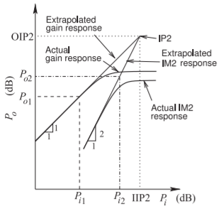
Figure \(\PageIndex{1}\): Output power versus input power of an amplifier plotted on a logarithmic scale. The IM2 response is a result of two-tone intermodulation (or of harmonic generation), and the input power is the power of each of the two signals that have equal amplitude. Extrapolations of the \(1:1\) linear fundamental response and the \(2:1\) second-order response intersect at the IP2 point.

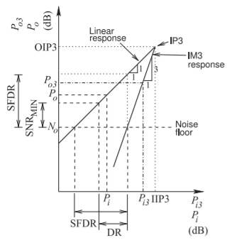
Figure \(\PageIndex{2}\): Output power versus input power of a stage or system plotted as output power in decibels versus input power in decibels. The IM3 response is a result of two-tone intermodulation, and the input power is the combined power of the two signals that have equal amplitude. Extrapolations of the \(1:1\) linear fundamental response and the \(3:1\) third-order intermodulation response intersect at the IP3 point.

signal (MDS) (also called the minimum detectable signal) is used instead of the noise floor. MDS is higher than the level of the noise floor by the minimum acceptable SNR (SNR\(_{\text{MIN}}\)). SNR\(_{\text{MIN}}\) is dependent on the type of modulation, on hardware inadequacies (captured by the implementation margin), on processing gain, and on the error correction coding used in a particular communications protocol.

It is interesting to note that the \(1\text{ dB}\) gain compression level has no effect on the dynamic range of microwave circuits and systems. This is because dynamic range is concerned with the ability to detect a signal when it is possible for the desired signal to be masked by spurious signals. Gain compression on its own does not introduce spurious signals so it does not interfere with the ability to detect a small signal.

The dynamic range does not relate to how accurately the sampled received signal matches the constellation diagram of the transmitted digitally modulated signal. Distortion of the constellation diagram is determined by noise, gain compression, and intermodulation distortion.

In the following, an expression for SFDR is developed in terms of input-referenced quantities, and this form of the SFDR is called the input referred SFDR (SFDR\(_{i}\)). A similarly referenced dynamic range (DR\(_{i}\)) is also developed.

Figure \(\PageIndex{2}\) graphically defines the dynamic ranges. The point of intersection of the extrapolated linear and IM3 responses is called the third-order intercept point (IP3 intercept). The point is identified by the output-referred intercept power (OIP3) or by the input-referred IP3 intercept power (IIP3) and these are key parameters in describing the linearity of nonlinear subsystems.

In the linear gain region, the output power \(P_{o}\) versus the input power \(P_{i}\) has a slope of \(1:1\), so that

\[\label{eq:1}P_{\text{dBm},i}=P_{\text{dBm},o}-G_{\text{dB}} \]

where \(G_{\text{dB}}\) is the power gain in decibels. \(P_{o}\) is used here as the output power, with \(P_{\text{dBm},o}\) indicating the output power in \(\text{dBm}\). \(P_{i}\) and \(P_{\text{dBm},i}\) are similarly defined. In terms of input quantities

\[\label{eq:2}\text{IIP3}=\frac{\text{OIP3}}{G}=\text{IIP3}_{\text{dBm}}=\text{OIP3}_{\text{dBm}}-G_{\text{dB}} \]

where again the \(\text{dBm}\) subscript indicates that the quantity is expressed in decibels referred to \(1\text{ mW}\).

The nonlinearity of RF active components results in harmonics and intermodulation components. With the narrowband amplifiers of communication and radar systems, output filters conveniently filter out harmonics. However, intermodulation distortion cannot be filtered out, as these components are within the main passband. The intermodulation components are therefore spurious tones. Generally just one of these defines the maximum spurious tone and nearly always it is one of the third-order intermodulation tones resulting from a two-tone input. Consideration of the maximum spurious tone and the noise floor defines the SFDR.

Examining Figure \(\PageIndex{2}\) leads to the following inequality describing the linear gain of the amplifier:

\[\begin{align}\frac{\text{OIP3}_{\text{dBm}}-P_{\text{dBm},o}}{\text{IIP3}_{\text{dBm}}-P_{\text{dBm},i}}&=\frac{\text{OIP3}_{\text{dBm}}-P_{\text{dBm},o}}{(\text{OIP3}_{\text{dBm}}-G_{\text{dB}})-P_{\text{dBm},i}}\nonumber \\ \label{eq:3}&=1\end{align} \]

The IM3 response is characterized by first introducing an equivalent input power, \(P_{\text{dBm},i3}\) (\(P_{i3}\) expressed in \(\text{dBm}\)), defined as the average power of the two-tone signal that generates an IM3 of power \(P_{\text{dBm},o3}\). Noting that \(P_{\text{dBm},o3}\) varies with a \(3:1\) logarithmic slope with respect to \(P_{\text{dBm},i3}\), then

\[\label{eq:4}\frac{\text{OIP3}_{\text{dBm}}-P_{\text{dBm},o3}}{(\text{OIP3}_{\text{dBm}}-G_{\text{dB}})-P_{\text{dBm},i3}}=3 \]

or

\[\label{eq:5}P_{\text{dBm},i3}=\frac{1}{3}(2\cdot\text{OIP3}_{\text{dBm}}+P_{\text{dBm},o3}-3G_{\text{dB}}) \]

The SFDR can now be defined when the third-order intermodulation product of two-tone excitation is the dominant spurious tone. The SFDR is defined as the difference between \(P_{i3}\) and \(P_{i}\) when they produce IM3 and linear output, respectively, that are both equal to the output noise power, \(N_{o}\) (see Figure \(\PageIndex{2}\)); that is, when \(P_{o} = P_{o3} = N_{o}\). Replacing \(P_{\text{dBm},o}\) in Equation \(\eqref{eq:5}\) with \(N_{o}\) gives

\[\label{eq:6}P_{\text{dBm},i3}=\frac{1}{3}(2\cdot\text{OIP3}_{\text{dBm}}+N_{\text{dBm},o}-3G_{\text{dB}}) \]

and

\[\label{eq:7}P_{\text{dBm},i}=N_{\text{dBm},o}-G_{\text{dB}} \]

Note that the difference between the linear output and the third-order intermodulation reduces as the input power increases above \(P_{i3}\). Thus the output-referred SFDR is

\[\begin{align}\text{SFDR}_{\text{dB},o}&=P_{\text{dBm},i3}-P_{\text{dBm},i}\nonumber \\ &=\frac{2}{3}\text{OIP3}_{\text{dBm}}+\frac{1}{3}N_{\text{dBm},o}-G_{\text{dB}}-N_{\text{dBm},o}+G_{\text{dB}}\nonumber \\ \label{eq:8}&=\frac{2}{3}(\text{OIP3}_{\text{dBm}}-N_{\text{dBm},o})\end{align} \]

So SFDR is \(2/3\)rds of the range in decibels from the noise intercept to the third order intercept point. A similar development defines the identical input-referred SFDR:

\[\label{eq:9}\text{SFDR}_{\text{dB},i}=\frac{2}{3}(\text{IIP3}_{\text{dBm}}-N_{\text{dBM},i}) \]

Note that \(N_{i}\) is the input-referred noise and includes noise applied to the module as well as the noise produced internally in the module and referred to the input. The SFDR provides a combined measure of distortion and noise. However, for usable dynamic range the minimum acceptable SNR must be considered. The minimum SNR (SNR\(_{\text{MIN}}\)) required is determined by the communication or radar modulation format, error coding, and acceptable BER. So in defining DR, the input power of the desired signal must increase sufficiently to produce an SNR of at least SNR\(_{\text{MIN}}\). Since the desired spurious level is still at the noise floor, this implies a direct subtraction in decibels of the desired SNR. Therefore the input-referred third-order dynamic range, preferred for receivers, is

\[\label{eq:10}\text{DR}_{i}=\frac{2}{3}(\text{IIP3}_{\text{dBm}}-N_{\text{dBm},i}-\text{SNR}_{\text{dB, MIN}}) \]

and the output-referred dynamic range, preferred for transmitters, is

\[\label{eq:11}\text{DR}_{o}=\frac{2}{3}(\text{OIP3}_{\text{dBm}}-N_{\text{dBm},o}-\text{SNR}_{\text{MIN}}) \]

The minimum discernible signal at the output is

\[\label{eq:12}\text{MDS}_{\text{dBm},o}=N_{\text{dBm},o}+\text{SNR}_{\text{dB},\text{MIN}} \]

so the output-referred dynamic range can be written as

\[\label{eq:13}\text{DR}_{o}=\frac{2}{3}(\text{OIP3}_{\text{dBm}}-\text{MDS}_{\text{dBm},o}) \]

So DR is \(2/3\)rds of the range in decibels from the level of the minimum detectable signal to the third order intercept point. The minimum discernible signal at the input is

\[\label{eq:14}\text{MDS}_{\text{dBm},i}=N_{\text{dBm},i}+\text{SNR}_{\text{dB, MIN}} \]

and the input-referred dynamic range (equal to \(\text{DR}_{o}\)) can be written as

\[\label{eq:15}\text{DR}_{i}=\frac{2}{3}(\text{IIP3}_{\text{dBm}}-\text{MDS}_{\text{dBm},i}) \]