6.2: Mixer

Frequency conversion, mixing or heterodyning, is the process of converting information at one frequency (present in the form of a modulated carrier) to another frequency. The second frequency is either higher, in the case of frequency up-conversion, where it is more easily transmitted, or lower, when mixing is called frequency down-conversion, where it is more easily captured. The mixer types are shown in Figure \(\PageIndex{1}\). Capture of the down-converted signal is nearly always by an ADC. Frequency conversion can occur with any nonlinear element.

Consider the information signal flow in the down-converter in Figure \(\PageIndex{1}\)(a). (A similar discussion applies to the up-converter in Figure \(\PageIndex{1}\)(b).) From the left, a modulated RF signal centered at \(f_{\text{RF}}\) is presented to a mixer that is pumped by a large LO signal at \(f_{\text{LO}}\). The intended function of the mixer is to convert the information on the modulated RF to a lower intermediate frequency (IF) centered at \(f_{\text{IF}} = |f_{\text{RF}} − f_{\text{LO}}|\). The spectrum of the mixer, shown on the right on Figure \(\PageIndex{1}\)(a), has another tone, \(f_{\text{IM}}\) called the image tone. The image at \(f_{\text{IM}}\) is an interferer, as it is also down-converted to the IF since \(f_{\text{IF}} = |f_{\text{IM}} − f_{\text{LO}}|\). Noise at the image is also down-converted to the IF. For the up-converter the high-power noise coming from the power amplifier at the image would be transmitted. Mixer design therefore must consider how image and noise are handled, as well as the efficiency of the conversion process.

In Figure \(\PageIndex{2}\)(a) a nonlinear device is driven by two signals at \(\omega_{M}\) and \(\omega_{C}\). The larger signal, the LO, is also called the pump and the other signal is called the RF. The spectrum of the signals present in the circuit is shown in Figure \(\PageIndex{2}\)(c). In this mixer the aim is to produce a signal at the difference frequency (or IF) with the same modulation, and hence the same information, as the original RF signal. The transistor mixer shown in Figure \(\PageIndex{3}\) uses filtering to separate the RF, LO, and IF components.

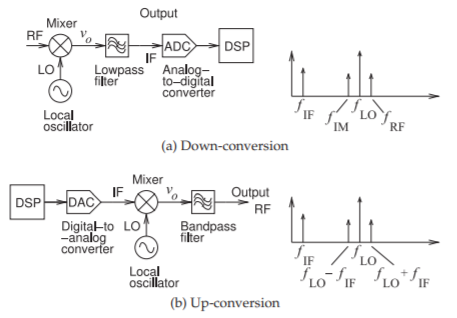
Figure \(\PageIndex{1}\): Frequency conversion using a mixer.

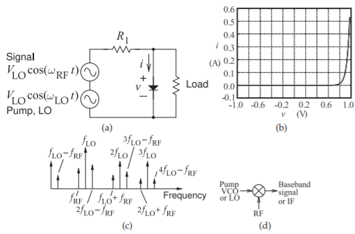
Figure \(\PageIndex{2}\): Diode mixer: (a) circuit; (b) diode current-voltage characteristic; (c) spectrum across the nonlinear device; and (d) schematic symbol for a mixer.

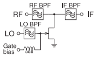
Figure \(\PageIndex{3}\): Single-ended FET mixer with LO, RF, and IF bandpass filters.

6.2.1 Mixer Analysis

A mixer can be designed around any nonlinear device [1]. Using an operational amplifier, an ideal multiplier can be designed that will multiply two signals, each described as cosinusoids. If the LO cosinusoid is \(\cos(\omega_{1}t)\) and the input RF cosinusoid is \(\cos(\omega_{2}t)\), the multiplication of the two signals will produce an output (using the trigonometric identity \(\cos(A) \cos(B) = \frac{1}{2} [\cos(A − B) + \cos(A + B)])\):

\[\begin{align}y(t)&=[\cos(\omega_{1}t)]\cdot [\cos(\omega_{2}t)]\nonumber \\ \label{eq:1}&=\frac{1}{2}\left\{\cos[(\omega_{1}-\omega_{2})t]+\cos[(\omega_{1}+\omega_{2})t]\right\}\end{align} \]

This has two components: one at the radian frequency \((\omega_{1} −\omega_{2})\) and the other at \((\omega_{1} +\omega_{2})\). If the LO and RF signal are close, then the component at \((\omega_{1} −\omega_{2})\) will be at a frequency much lower than either the LO or the RF, and the component at \((\omega_{1} +\omega_{2})\) will be at almost twice the input frequencies. Appropriate filtering will choose one of these components depending on whether the application is up-conversion or down-conversion. At microwave frequencies, circuits that do not realize ideal multiplication must be used. This section considers what happens when two components are applied to an arbitrary nonlinearity described by a low-order polynomial. The result is that a large number of tones will be generated in the mixing process. Balanced circuit designs can significantly reduce many of these tones, greatly reducing the filtering required to select a particular output.

A two-tone input

\[x(t) = |X_{1}| \cos(\omega_{1}t +\phi_{1}) + |X_{2}| \cos(\omega_{2}t +\phi_{2})\nonumber \]

can be written using complex notation as

\[x(t) = \frac{1}{2}[X_{1}\text{e}^{\jmath\omega_{1}t} + X_{1}^{\ast}\text{e}^{−\jmath\omega_{1}t} + X_{2}\text{e}^{\jmath\omega_{2}t} + X_{2}^{\ast}\text{e}^{−\jmath\omega_{2}t}] \nonumber \]

Note that the coefficient of the positive exponential frequency component is one-half that of the phasor. Thus the phasor of the \(\omega_{1}\) component is \(X_{1} = |X_{1}|\text{e}^{(\jmath\phi_{1})}\) and the phasor of the \(\omega_{2}\) component is \(X_{2} = |X_{2}|\text{e}^{(\jmath\phi_{2})}\). The first three powers of \(x\) can be easily expanded manually; for example, expanding \(x^{2}\) gives

\[\begin{align}x^{2}(t)&=\left(\frac{1}{2}\right)^{2}\left[X_{1}^{2}\text{e}^{\jmath 2\omega_{1}t}+2X_{1}X_{1}^{\ast}+2X_{1}X_{2}\text{e}^{\jmath(\omega_{1}+\omega_{2})t} +2X_{1}X_{2}^{\ast}\text{e}^{\jmath(\omega_{1}-\omega_{2})t}\right.\nonumber\\ &\quad +(X_{1}^{\ast})^{2}\text{e}^{-\jmath 2\omega_{1}t}+2X_{1}^{\ast}X_{2}\text{e}^{\jmath(\omega_{2}-\omega_{1})t}+2X_{1}^{\ast}X_{2}^{\ast}\text{e}^{-\jmath(\omega_{1}+\omega_{2})t}+X_{2}^{2}\text{e}^{\jmath 2\omega_{2}t}\nonumber \\ \label{eq:2}&\quad \left. +2X_{2}X_{2}^{\ast}+(X_{2}^{\ast})^{2}\text{e}^{-\jmath 2\omega_{2}t}\right] \end{align} \]

and similarly, expanding \(x^{3}\) yields

\[\begin{align} x^{3}(t)&=\left(\frac{1}{2}\right)^{3}\left[X_{1}^{3}\text{e}^{\jmath 3\omega_{1}t}+3X_{1}^{2}X_{1}^{\ast}\text{e}^{\jmath\omega_{1}t}+3X_{1}^{2}X_{2}\text{e}^{\jmath(2\omega_{1}+\omega_{2})t}\right.\nonumber \\ &\quad +3X_{1}^{2}X_{2}^{\ast}\text{e}^{\jmath(2\omega_{1}-\omega_{2})t}+3X_{1}(X_{1}^{\ast})^{2}\text{e}^{-\jmath\omega_{1}t}+6X_{1}X_{1}^{\ast}X_{2}\text{e}^{\jmath\omega_{2}t}\nonumber \\ &\quad +6X_{1}X_{1}^{\ast}X_{2}^{\ast}\text{e}^{-\jmath\omega_{2}t}+3X_{1}X_{2}^{2}\text{e}^{\jmath(\omega_{1}+2\omega_{2})t}\nonumber \\ &\quad +6X_{1}X_{2}X_{2}^{\ast}\text{e}^{\jmath\omega_{1}t}+3X_{1}(X_{2}^{\ast})^{2}\text{e}^{\jmath(\omega_{1}-2\omega_{2})t}+(X_{1}^{\ast})^{3}\text{e}^{-\jmath 3\omega_{1}t}\nonumber \\ &\quad +3(X_{1}^{\ast})^{2}X_{2}\text{e}^{\jmath(\omega_{2}-2\omega_{1})t}+3(X_{1}^{\ast})^{2}X_{2}^{\ast}\text{e}^{-\jmath(2\omega_{1}+\omega_{2})t}+3X_{1}^{\ast}X_{2}^{2}\text{e}^{\jmath (2\omega_{2}-\omega_{1})t}\nonumber \\ &\quad +3X_{1}^{\ast}(X_{2}^{\ast})^{2}\text{e}^{-\jmath (\omega_{1}+2\omega_{2})t}+X_{2}^{3}\text{e}^{\jmath 3\omega_{2}t}+6X_{1}^{\ast}X_{2}^{\ast}X_{2}\text{e}^{-\jmath\omega_{1}t}\nonumber \\ \label{eq:3}&\quad \left.+3X_{2}^{2}X_{2}^{\ast}\text{e}^{\jmath\omega_{2}t}+3X_{2}(X_{2}^{\ast})^{2}\text{e}^{-\jmath\omega_{2}t}+(X_{2}^{\ast})^{3}\text{e}^{-\jmath 3\omega_{2}t}\right] \end{align} \]

so that the output of the cubic equation,

\[y(t)=a_{0}+a_{1}x(t)+a_{2}x^{2}(t)+a_{3}x^{3}(t)\nonumber \]

can be calculated for a two-tone input. Table \(\PageIndex{1}\) lists these phasors and groups them by frequency. A more general approach is described in [2].

The phasors of the various intermodulation products resulting from \(x,\: x^{2},\) and \(x^{3}\) can be taken as the coefficients of the positive exponential frequency components after the factor of two correction required for terms other than DC [2]. Terms of the same frequency are summed to obtain the output at a particular frequency. For example, the phasor output at \((2\omega_{1} −\omega_{2})\) is given by the sum of three intermodulation products:

\[\label{eq:4}Y_{(2\omega_{1}-\omega_{2})}=a_{3}\left(\frac{3}{4}\right)X_{1}^{2}X_{2}^{\ast} \]

So the level of the output of a mixer, here \(Y_{(2\omega_{1}−\omega_{2})}\) at radian frequency \((2\omega_{1}−\omega_{2})\), is related directly to the strength of the LO signal (with amplitude \(|X_{1}|\)), the strength of the nonlinearity (captured by the \(a_{n}\) coefficients), and the level of the input signal \(|X_{2}|\). Unfortunately, low-order power series analysis as used here is not sufficient to model practical mixers, and computer-aided modeling tools are necessary. However, the manual analysis enables operation to be understood and architectures to be developed that intrinsically have the desired characteristics.

Intermodulation product	Frequency	Order
\(\begin{array}{c}{\frac{1}{2}X_{1}X_{1}^{\ast}}\\{\frac{1}{2}X_{2}X_{2}^{\ast}}\end{array}\)	\(\begin{array}{c}{0}\\{0}\end{array}\)	\(\begin{array}{c}{2}\\{2}\end{array}\)
\(\begin{array}{c}{2\frac{1}{2}X_{1}=X_{1}}\\{2(\frac{1}{2})^{3}3X_{1}^{2}X_{1}^{\ast}=\frac{3}{4}X_{1}^{2}X_{1}^{\ast}}\\{2(\frac{1}{2})^{3}6X_{1}X_{2}X_{2}^{\ast}=\frac{3}{2}X_{1}X_{2}X_{2}^{\ast}}\end{array}\)	\(\begin{array}{c}{\omega_{1}}\\{\omega_{1}}\\{\omega_{1}}\end{array}\)	\(\begin{array}{c}{1}\\{3}\\{3}\end{array}\)
\(\begin{array}{c}{2\frac{1}{2}X_{2}=X_{2}}\\{2(\frac{1}{2})^{3}3X_{2}^{2}X_{2}^{\ast}=\frac{3}{4}X_{2}^{2}X_{2}^{\ast}}\\{2(\frac{1}{2})^{3}6X_{1}X_{1}^{\ast}X_{2}=\frac{3}{2}X_{1}X_{1}^{\ast}X_{2}}\end{array}\)	\(\begin{array}{c}{\omega_{2}}\\{\omega_{2}}\\{\omega_{2}}\end{array}\)	\(\begin{array}{c}{1}\\{3}\\{3}\end{array}\)
\(2(\frac{1}{2})^{2}X_{1}^{2}=\frac{1}{2}2X_{1}^{2}\)	\(2\omega_{1}\)	\(2\)
\(2(\frac{1}{2})^{2}X_{2}^{2}=\frac{1}{2}2X_{2}^{2}\)	\(2\omega_{2}\)	\(2\)
\(2(\frac{1}{2})^{3}X_{1}^{3}=\frac{1}{4}X_{1}^{3}\)	\(3\omega_{1}\)	\(3\)
\(2(\frac{1}{2})^{3}X_{2}^{3}=\frac{1}{4}X_{2}^{3}\)	\(3\omega_{2}\)	\(3\)
\(2\frac{1}{2}X_{1}X_{2}=X_{1}X_{2}\)	\(\omega_{1}+\omega_{2}\)	\(2\)
\(2\frac{1}{2}X_{1}X_{2}^{\ast}=X_{1}X_{2}^{\ast}\)	\(\omega_{1}-\omega_{2}\)	\(2\)
\(2(\frac{1}{2})^{3}3X_{1}^{2}X_{2}=\frac{3}{4}X_{1}^{2}X_{2}\)	\(2\omega_{1}+\omega_{2}\)	\(3\)
\(2(\frac{1}{2})^{3}3X_{1}^{2}X_{2}^{\ast}=\frac{3}{4}X_{1}^{2}X_{2}^{\ast}\)	\(2\omega_{1}-\omega_{2}\)	\(3\)
\(2(\frac{1}{2})^{3}3X_{1}X_{2}^{2}=\frac{3}{4}X_{1}X_{2}^{2}\)	\(\omega_{1}+2\omega_{2}\)	\(3\)
\(2(\frac{1}{2})^{3}3X_{1}^{\ast}X_{2}^{2}=\frac{3}{4}X_{1}^{\ast}X_{2}^{2}\)	\(2\omega_{2}-\omega_{1}\)	\(3\)

Table \(\PageIndex{1}\): The intermodulation products resulting from \(x,\: x^{2}\), and \(x^{3}\), where \(x\) is a two-tone signal, showing only the positive frequencies. The first column gives the complex amplitudes (phasors) of the frequency components. (The order is the power of \(x\).)

6.2.2 Mixer Performance Parameters

The main characteristics that define the performance of a mixer are the conversion gain or loss, and the noise figure [3, 4]. Mixing results from a nonlinear process that generates many tones and not just the ones of interest. Consequently, additional parameters are used to describe the performance of a mixer, and these derive from the generation of the additional tones. The mixer performance parameters are as follows:

Conversion loss: This is the ratio of the available power of the input signal to that of the output signal after mixing. It is usually expressed in decibels. In the diode mixer shown in Figure \(\PageIndex{5}\), the conversion loss is

\[\label{eq:5}L_{C}=\frac{P_{\text{in}}(\text{RF})}{P_{\text{out}}(\text{IF})} \]

In decibels, the conversion loss is

\[\label{eq:6}L_{C}|_{\text{dB}}=10\log_{10}\left[\frac{P_{\text{in}}(\text{RF})}{P_{\text{out}}(\text{IF})}\right] \]

Noise figure (NF): The NF is \(10\) times the log of the noise factor \(F\). The noise factor is the ratio of the SNR at the RF input to the SNR at the IF output (using the input noise generated by a resistor at standard temperature, \(290\text{ K}\)).

However, there are qualifications for mixers. The first is that two inputs (at the RF and image frequencies) can produce noise and signal power at the IF. The double-sideband (DSB) NF includes signal and noise contributions from both the RF and the image frequencies. This is the situation with radiometry and astronomy, where the signal is at both sidebands. Single-sideband (SSB) NF includes the input signal at the RF only, but includes noise originating at both the RF and at the image frequencies. This is the situation for mixers in communications where the signal is only at one sideband.

Mixers can have substantial excess noise, as noise that is offset in frequency from the LO and its harmonics by the magnitude of the IF frequency will be down-converted to the IF for a down-converter, or converted to the RF in an up-converter. This process is sometimes called noise folding.

In summary, two noise figures are used with mixers, SSB NF and DSB NF. Which to use depends on the system in which the mixer is embedded.

Image rejection: If a mixer has an LO of \(1.1\text{ GHz}\) and an RF of \(1.5\text{ GHz}\), then the IF will be at \(400\text{ MHz}\). This IF can also be generated by the image signal at \(700\text{ MHz}\). Numerically the image is the reflection of the RF in the LO. Image rejection refers to the ability of a mixer to reject the image signal. This can be achieved, for example, by using an input RF bandpass filter.

If the applied image and intended signal powers are the same and the level of the output signal (at the IF) produced by the intended RF signal is \(P_{\text{out}}\), and that produced by the image signal is \(P_{\text{out,image}}\), then the image rejection ratio (IRR) is

\[\label{eq:7}\text{IRR}=\frac{P_{\text{out}}}{P_{\text{out, image}}} \]

This is typically expressed in decibels and

\[\label{eq:8}\text{IRR}|_{\text{dB}}=10\log_{10}\left(\frac{P_{\text{out}}}{P_{\text{out, image}}}\right) \]

Example \(\PageIndex{1}\): Mixer Calculations

A mixer has an LO of \(10\text{ GHz}\). The mixer is used to convert a signal at \(10.1\text{ GHz}\) to an IF at \(100\text{ MHz}\), and has a conversion loss, \(L_{c}\) of \(3\text{ dB}\) and an image rejection of \(20\text{ dB}\). Two signals are presented to the mixer, one at \(10.1\text{ GHz}\) with a power of \(100\text{ nW}\) and the other at \(9.9\text{ GHz}\) with a power of \(1\:\mu\text{W}\).

1. What is the output power of the (intended) signal at the IF?
2. What is the signal-to-interference ratio at the IF (ignoring noise)?

Solution

1. \(L_{c} = 3\text{ dB} = 2\) and from Equation \(\eqref{eq:5}\) the output power at IF of the intended signal is
   \[\label{eq:9}P_{\text{out}}=P_{\text{in}}(\text{RF})/L_{c}=100\text{ nW}/2=50\text{ nW}=-43\text{ dBm} \]
2. Interference at the IF comes from the down-converted image signal. \(\text{IRR} = 20\text{ dB} = 100\). If the applied powers of the intended signal and the image signal are the same, from Equation \(\eqref{eq:7}\),
   \[\label{eq:10}\text{IRR}=\frac{P_{\text{out}}}{P_{\text{out, image}}}\quad\text{i.e.}\quad P_{\text{out, image}}=\frac{P_{\text{out}}}{\text{IRR}} \]
   This must be modified to account for the difference in the applied power levels and
   \[P_{\text{out, image}}=\frac{P_{\text{out}}}{\text{IRR}}\frac{P_{\text{in}}(\text{RF, image})}{P_{\text{in}}(\text{RF})}=\frac{(50\text{ nW})\cdot (1\:\mu\text{W})}{100\cdot (100\text{ nW})}=\frac{(50\text{ nW})\cdot (1000\text{ nW})}{100\cdot (100\text{ nW})}=5\text{ nW}\nonumber \]
   The signal-to-interference ratio is
   \[\label{eq:11}\text{SIR}=\frac{P_{\text{out}}}{P_{\text{out, image}}}=\frac{50\text{ nW}}{5\text{ nW}}=10=10\text{ dB} \]

6.2.3 Mixer Waveforms

This section presents the waveforms of diode mixers. Diode mixers, such as the balanced mixer in Figure \(\PageIndex{4}\), are bilateral. In a communication transceiver such a mixer can be used for both the receive and transmit functions, greatly simplifying filtering requirements. Most mixers in cell phones, however, are based on transistors, but the underlying architecture corresponds to a single-diode mixer or, more commonly, the diode ring double-balanced mixer.

The first mixer to be considered is the single-ended mixer shown in Figure \(\PageIndex{5}\)(a). Filters are not included thus revealing the full complexity of the spectra. The transient waveform across the diode (measured at the test point) is shown in Figure \(\PageIndex{5}\)(b). The turn-on transient is due to both the turn-on ramp of the LO and RF sources, and to the internal capacitance of the diode. The spectra of the signal at the test point is shown in Figure \(\PageIndex{5}\)(c and d). The desired signal here is the IF, which is at the difference frequency of the LO and RF (i.e., at \(400\text{ MHz}\)). Extracting just the IF in the response shown in Figure \(\PageIndex{5}\)(d) would require significant filtering. The level of the IF tone here is \(11.5\text{ mV}_{\text{peak}}\). If a lossless \(400\text{ MHz}\) filter is attached to the test point and the IF load (on the other side of the filter) is \(50\:\Omega\), the IF power delivered to the load is \(P_{\text{out}} = \frac{1}{2}(11.5\text{ mV})^{2}/(50\:\Omega) = 1.322\:\mu\text{W}\). The available RF power is \(P_{\text{in}} =\frac{1}{2}(100\text{ mV})^{2}/(50\:\Omega) = 100\:\mu\text{W}\). So the conversion loss is

\[\label{eq:12}L_{C}=\frac{100\:\mu\text{W}}{1.332\:\mu\text{W}}=75.08=18.8\text{ dB} \]

Now consider the diode ring mixer shown in Figure \(\PageIndex{6}\). Waveforms and spectra at the LO, IF, and RF test points are shown in Figure \(\PageIndex{7}\). Note how relatively clean the spectra are at each of the test points. The reduction in clutter is the result of the balanced circuit. The circuit in Figure \(\PageIndex{6}\) is known as a double-balanced mixer, and the same concept can be used with transistor mixers.

Focusing on just the spectra at the IF test point (Figure \(\PageIndex{7}\)(e)), it can be seen that the LO signal and its harmonics are nonexistent. The components other than the \(400\text{ MHz}\) IF are other sum and difference products of the RF and LO. However, compared to the spectra of the single-ended diode mixer

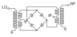
Figure \(\PageIndex{4}\): Diode ring double-balanced mixer.

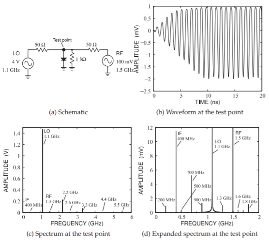
Figure \(\PageIndex{5}\): Single-ended diode mixer.

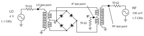
Figure \(PageIndex{6}\): Diode double-balanced mixer schematic.

in Figure \(\PageIndex{5}\)(c and d), many of these are eliminated as well. This is a very attractive circuit, as it significantly reduces the specifications required for an output filter. This is one of the special characteristics of RF and microwave design. Much can be gained by being creative—a designer gets better with experience. The level of the IF signal at the RF test point is \(26.7\text{ mV}_{\text{peak}}\). The IF power delivered to the \(50\:\Omega\) load is \(P_{\text{out}} = \frac{1}{2} (26.7\text{ mV})^{2}/(50\:\Omega) = 7.126\:\mu\text{W}\). The available RF power is \(P_{\text{in}} = \frac{1}{2} (100\text{ mV})^{2}/(50\:\Omega) = 100\:\mu\text{W}\). So the conversion loss is

\[\label{eq:13}L_{C}=\frac{100\:\mu\text{W}}{7.126\:\mu\text{W}}=14.02=11.47\text{ dB} \]

The conversion loss is much lower than was obtained with the single-ended mixer. In part this is because power was not dissipated in a large number of spurious tones.

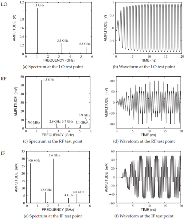
Figure \(\PageIndex{7}\): Waveforms and spectra of the double-balanced diode ring mixer of Figure \(\PageIndex{6}\).

6.2.4 Switching Mixer

The analysis of a mixer in Section 6.2.1 modeled the mixing element using a polynomial. With a large LO, an alternative view of a mixer is to consider it as a switching device in which the conductance of the mixing element is periodically switched by the LO.

A simple switching diode mixer is shown in Figure \(\PageIndex{8}\)(a). If the LO level is large, then the mixer can be modeled by the equivalent circuit shown in Figure \(\PageIndex{8}\)(b) with a periodically varying conductance, \(g_{\text{LO}}(t)\). This is a square wave with the same frequency and period as the applied LO sinewave. The diode effectively looks like a switch with the conductance alternating between a maximum value \(g_{m}\) and zero (see Figure \(\PageIndex{8}\)(c)). The first few terms of the Fourier series expansion of \(g_{\text{LO}}(t)\) are

\[\label{eq:14}g_{\text{LO}}(t)=g_{m}\left[\frac{1}{2}+\frac{1}{\pi}\cos(\omega_{\text{LO}}t)+\frac{2}{3\pi}\cos(3\omega_{\text{LO}}t)+\ldots\right] \]

The small RF signal interacts with the switching conductance so that the output current is

\[\label{eq:15}i(t)=g_{\text{LO}}(t)[v_{\text{RF}}-i_{x}(t)R] \]

Ignoring \(R\), then the IF current, where \(\omega_{\text{IF}} = \omega_{\text{RF}} −\omega_{\text{LO}}\), at the point \(\mathsf{x}\) is

\[\begin{align}i_{\text{IF}}(t)&=g_{\text{LO}}(t)v_{\text{RF}}(t)=\frac{g_{m}}{\pi}\cos(\omega_{\text{LO}}t)v_{\text{RF}}\cos(\omega_{\text{RF}}t) \nonumber \\ \label{eq:16} &=\frac{g_{m}v_{\text{RF}}}{2\pi}\{\cos[(\omega_{\text{LO}}-\omega_{\text{RF}})t]+\cos[(\omega_{\text{LO}}+\omega_{\text{RF}})t]\}\end{align} \]

Typically the IF signal at \((\omega_{\text{LO}} −\omega_{\text{RF}})\) would be extracted through a bandpass or lowpass filter that allows only the IF component to pass and an IF voltage is realized as the current passes through a load resistor.

One of the advantages of the switching mixer is that performance is relatively insensitive to the level of the LO. The LO could be a sinewave and still the variation of the conductance would be close to being a square wave. So then the design of the mixer specifically is to develop a square variation of the conductance.

Switching mixers can be realized using other circuits. One of these is the diode ring mixer shown in Figure \(\PageIndex{9}\). Here the center-tapped transformers produce differential LO and RF signals. The large LO is transformed by the tapped transformer to produce a large differential signal that turns pairs of diodes on in sequence. During the positive half of the LO cycle, the

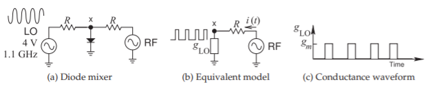
Figure \(\PageIndex{8}\): Switching diode mixer; \(g_{\text{LO}}\) is a conductance.

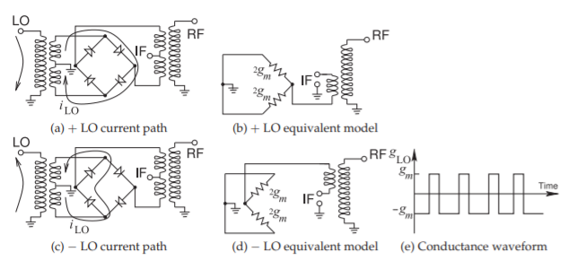
Figure \(\PageIndex{9}\): Diode ring mixer as a switching mixer. \(g_{m}\) is a conductance.

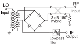
Figure \(\PageIndex{10}\): Diode ring mixer implemented using a hybrid to produce a pseudo-balanced signal.

two right-hand diodes in Figure \(\PageIndex{9}\)(a) pass current limited by the source impedance of the LO source and each diode has a conductance \(2g_{m}\), as seen in Figure \(\PageIndex{9}\)(b). During the negative half-cycle of the LO, the left-hand diodes pass current and each has conductance \(2g_{m}\), see Figure \(\PageIndex{9}\)(c and d). When not forward biased, the diodes appear as open circuits. This process results in the conductance waveform shown in Figure \(\PageIndex{9}\)(e). An important characteristic of this waveform is that it is symmetrical even when nonidealities are considered.

An RF implementation of the diode mixer is shown in Figure \(\PageIndex{10}\). The \(180^{\circ}\) hybrid replaces the transformer to distribute oppositely phased RF signals to the diode ring. The IF is now taken from the center tap of the LO transformer and is passed through a lowpass filter to remove all signals other than the IF. This is a down-converting mixer. If the mixer is an up-converting mixer, then the lowpass filter would be replaced by a bandpass filter.

Transistor-based mixer implementations using the ring mixer concept are shown in Figure \(\PageIndex{11}\). These circuits are used in monolithic ICs with the differential signals available from preceding stages and the IF output is also differential. The transistors operate as switches that are controlled by the LO signal and the conductance waveform is as for the diode mixer (i.e., as in Figure \(\PageIndex{9}\)(e)). Another switching mixer is the transistor commutating mixer shown in Figure \(\PageIndex{12}\).

Traditionally the the biggest issue with switching mixers was is the substantial LO power required and the limited dynamic range of the mixer in

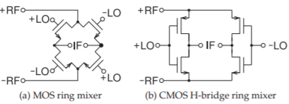
Figure \(\PageIndex{11}\): Transistor ring mixers.

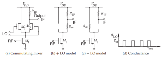
Figure \(\PageIndex{12}\): Commutating transistor mixer.

converting RF to IF (for a down-converter) or IF to RF (for an up-converter). This situation changes with the \(32\text{ nm}\) and lower CMOS processing nodes. This has resulted in CMOS switching mixers being important elements of RFICs and these have superior dynamic range.

6.2.5 Subharmonic Mixer

If the nonlinear element of a mixer is particularly strong, or perhaps the drive level is very high, mixing will occur when the frequency of the LO drive of the mixer is a subharmonic of the the effective LO frequency. Consider the switching mixers discussed in Section 6.2.4 and the switching conductance, Figure \(\PageIndex{12}\)(c), of the commutating mixer in Figure \(\PageIndex{12}\)(a). With this mixer the RF signal effectively mixes with an harmonic of the applied LO. Here these harmonics are odd harmonics and so a commutating mixer driven by an LO signal at \(5\text{ GHz}\) will down-convert and RF signal at \(15.1\text{ MHz}\) to an IF frequency of \(100\text{ MHz}\). One of the advantages of a subharmonic mixer is that there is not a large \(15\text{ GHz}\) signal which could be a problem as it could leak into the front of a receiver and possibly radiate unintentionally. Another advantage is that with a conventional down-conversion mixing approach where the LO and RF are close in frequency, an LO at \(15\text{ GHz}\), in previous example, would need to be generated from the \(5\text{ GHz}\) signal. This would consume considerable power. So it could be more power efficient to use a subharmonic mixer rather than a frequency tripler and a conventional mixer. A subharmonic mixer could be the preferred design option especially for down-converting millimeter-wave signals. At high millimeter-wave frequencies (e.g. \(> 200\text{ GHz}\)) the mixer is often a passive nonlinear element.