1.6: RF Power Calculations

1.6.1 RF Propagation

As an RF signal propagates away from a transmitter the power density reduces conserving the power in the EM wave. In the absence of obstacles and without atmospheric attenuation the total power passing through the surface of a sphere centered on a transmitter is equal to the power transmitted. Since the area of the sphere of radius \(r\) is \(4πr^{2}\), the power density, e.g. in \(\text{W/m}^{2}\), at a distance \(r\) drops off as \(1/r^{2}\). With obstacles the EM wave can diffract, reflect, and follow multiple paths to a receiver where it can combine destructively or constructively. It is the destructive interference that is of concern as this limits the reliable reception of a signal. There is a low probability of perfect cancelation occurring and instead it is found that the power density reduces as \(1/r^{n}\) where \(n\) ranges from \(2\) for free space to \(5\) for a dense urban environment with many obstacles, no line of sight, and multiple signal paths.

Example \(\PageIndex{1}\): Signal Propagation

A signal is received at a distance \(r\) from a transmitter and the received power drops off as \(1/r^{2}\). When \(r = 1\text{ km}\), \(100\text{ nW}\) is received. What is \(r\) when the received power is \(100\text{ fW}\)?

Solution

The signal collected by the receiver is proportional to the power density of the EM signal. The received signal power \(P_{r} = k/r^{2}\) where \(k\) is a constant. This leads to

\[\label{eq:1}\frac{P_{r}(1\text{ km})}{P_{r}(r)}=\frac{100\text{ nW}}{100\text{ fW}}=10^{6}=\frac{kr^{2}}{k(1\text{ km})^{2}}=\frac{r^{2}}{(10^{3}\text{ m})^{2}};\quad r=\sqrt{10^{12}\text{ m}^{2}}=1000\text{ km} \]

Example \(\PageIndex{2}\): Signal Propagation With Obstructions

A transmitter sends a signal to a receiver in a suburban environment that is a distance \(d\) away. When \(d = 5\text{ km}\) the signal power received is \(100\text{ nW}\). At what distance from the transmitter is the reliably received signal \(1\text{ pW}\) if the received signal power falls off as \(1/d^{3}\).

Solution

Note that the signal falls off faster than the \(1/d^{2}\) variation of free space. It is not sufficient to know the total power transmitted and instead the power density at a particular distance must be known. The power reliably received, \(P_{R}\)(\(5\text{ km}\)), at \(5\text{ km}\) is \(100\text{ nW}\) and this is the power density, \(P_{D}\)(\(5\text{ km}\)), multiplied by the effective area, \(A_{r}\), of the receive antenna:

\[P_{R}\:(5\text{ km})=100\text{ nW}=P_{D}\: (5\text{ km})A_{r}=\frac{k}{d^{3}}=\frac{k}{(5\text{ km})^{3}}=\frac{k}{125\text{ km}^{3}}\nonumber \]

Both \(A_{r}\) and \(k\) are constants and \(k = 12500\text{ nW}\cdot\text{km}^{3} = 1.25\cdot 10^{−5}\text{ W}\cdot\text{km}^{3}\). The power received at a distance \(d\) is \(1\text{ pW}\) when

\[\begin{align} P_{R}(d)&=1\text{ pW}=10^{-12}\text{ W}=\frac{k}{d^{3}}=\frac{1.25\times 10^{-5}\text{W}\cdot\text{km}^{3}}{d^{3}}\nonumber \\ \label{eq:2} d^{3}&=\frac{1.25\times 10^{-5}\text{ W}\times\text{km}^{3}}{10^{-12}\text{ W}}=1.25\times 10^{7}\text{ km}^{3};\quad d=\sqrt[3]{1.25\times 10^{7}}\text{ km}=232.1\text{ km}\end{align} \]

Description	Formula	Example
Equivalence	\(y=\log_{b}(x)\longleftrightarrow x=b^{y}\)	\(\log (1000)=3\text{ and }10^{3}=1000\)
Product	\(\log_{b}(xy)=\log_{b}(x)+\log_{b}(y)\)	\(\log (0.13\cdot 978)=\log (0.13)+\log (978)=-0.8861+2.990=2.104\)
Ratio	\(\log_{b}(x/y)=\log_{b}(x)-\log_{b}(y)\)	\(\ln (8/2)=\ln (8)-\ln (2)=3-1=2\)
Power	\(\log_{b}(x^{p})=p\log_{b}(x)\)	\(\ln (3^{2})=2\ln (3)=2\cdot 1.0986=2.197\)
Root	\(\log_{b}(\sqrt[p]{x})=\frac{1}{p}\log_{b}(x)\)	\(\log (\sqrt[3]{20})=\frac{1}{3}\log (20)=0.4337\)
Change of base	\(\log_{b}(x)=\frac{\log_{k}(x)}{\log_{k}(b)}\)	\(\ln (100)=\frac{\log (100)}{\log (2)}=\frac{2}{0.30103}=6.644\)

Table \(\PageIndex{1}\): Common logarithm formulas. In engineering \(\log x ≡ \log_{10} x\) and \(\ln x ≡ \log_{2} x\)

1.6.2 Logarithm

A cellular phone can reliably receive a signal as small as \(100\text{ fW}\) and the signal to be transmitted could be \(1\text{ W}\). So the same circuitry can encounter signals differing in power by a factor of \(10^{13}\). To handle such a large range of signals a logarithmic scale is used.

Logarithms are used in RF engineering to express the ratio of powers using reasonable numbers. Logarithms are taken with respect to a base \(b\) such that if \(x = b^{y}\), then \(y = \log_{b}(x)\). In engineering, \(\log (x)\) is the same as \(\log_{10}(x)\), and \(\ln (x)\) is the same as \(\log_{e}(x)\) and is called the natural logarithm \((e = 2.71828\ldots)\). Unfortunately in physics and mathematics (and in programs such as MATLAB), \(\log x\) means \(\ln x\), so be careful. Common formulas involving logarithms are given in Table \(\PageIndex{1}\).

1.6.3 Decibels

RF signal levels are usually expressed in terms of the power of a signal. While power can be expressed in absolute terms such as watts (\(\text{W}\)) or milliwatts (\(\text{mW}\)), it is much more useful to use a logarithmic scale. The ratio of two power levels \(P\) and \(P_{\text{REF}}\) in bels\(^{1}\) (\(\text{B}\)) is

\[\label{eq:3}P(B)=\log\left(\frac{P}{P_{\text{REF}}}\right) \]

where \(P_{\text{REF}}\) is a reference power. Here \(\log x\) is the same as \(\log_{10} x\). Human senses have a logarithmic response and the minimum resolution tends to be about \(0.1\text{ B}\), so it is most common to use decibels (\(\text{dB}\)); \(1\text{ B} = 10\text{ dB}\). Common designations are shown in Table \(\PageIndex{2}\). Also, \(1\text{ mW} = 0\text{ dBm}\) is a very common power level in RF and microwave power circuits where the \(\text{m}\) in \(\text{dBm}\) refers to the \(1\text{ mW}\) reference. As well, \(\text{dBW}\) is used, and this is the power ratio with respect to \(1\text{ W}\) with \(1\text{ W} = 0\text{ dBW} = 30\text{ dBm}\).

Working on the decibel scale enables convenient calculations using power numbers ranging from \(10\)s of \(\text{dBm}\) to \(−110\text{ dBm}\) to be used rather than numbers ranging from \(100\text{ W}\) to \(0.00000000000001\text{ W}\).

\(P_{\text{REF}}\)	Bell units	Decibel units
\(1\text{ W}\)	\(\text{BW}\)	\(\text{dBW}\)
\(1\text{ mW} = 10^{-3}\text{ W}\)	\(\text{Bm}\)	\(\text{dBm}\)
\(1\text{ fW} = 10^{-15}\text{ W}\)	\(\text{Bf}\)	\(\text{dBf}\)

Table \(\PageIndex{2}\)a: Common power designations (a) Reference power, \(P_{\text{REF}}\)

Power ratio	in \(\text{dB}\)
\(10^{-6}\)	\(-60\)
\(0.001\)	\(-30\)
\(0.1\)	\(-20\)
\(1\)	\(0\)
\(10\)	\(10\)
\(1000\)	\(30\)
\(10^{6}\)	\(60\)

Table \(\PageIndex{2}\)b: Common power designations (b) Power ratios in decibels (\(\text{dB}\))

Power	Absolute power
\(-120\text{ dBM}\)	\(10^{-12}\text{ mW} = 10^{-15}\text{ W} = 1\text{ fW}\)
\(0\text{ dBm}\)	\(1\text{ mW}\)
\(10\text{ dBm}\)	\(10\text{ mW}\)
\(20\text{ dBm}\)	\(100\text{ mW} = 0.1\text{ W}\)
\(30\text{ dBm}\)	\(1000\text{ mW} = 1\text{ W}\)
\(40\text{ dBm}\)	\(10^{4}\text{ mW} = 10\text{ W}\)
\(50\text{ dBm}\)	\(10^{5}\text{ mW} = 100\text{ W}\)
\(-90\text{ dBm}\)	\(10^{-9}\text{ mW} = 10^{-12}\text{ W} = 1\text{ pW}\)
\(-60\text{ dBm}\)	\(10^{-6}\text{ mW} = 10^{-9}\text{ W} = 1\text{ nW}\)
\(-30\text{ dBm}\)	\(0.001\text{ mW} = 1\:\mu\text{W}\)
\(-20\text{ dBm}\)	\(0.01\text{ mW} = 10\:\mu\text{W}\)
\(-10\text{ dBm}\)	\(0.1\text{ mW} = 100\:\mu\text{W}\)

Table \(\PageIndex{2}\)c: Common power designations (c) Powers in \(\text{dBm}\) and watts

Example \(\PageIndex{3}\): Power Gain

An amplifier has a power gain of \(1200\). What is the power gain in decibels? If the input power is \(5\text{ dBm}\), what is the output power in \(\text{dBm}\)?

Solution

Power gain in decibels, \(G_{\text{dB}} = 10 \log 1200 = 30.79\text{ dB}\).

The output power is \(P_{\text{out|dBm}} = P_{\text{dB}} + P_{\text{in|dBm}} = 30.79 + 5 = 35.79\text{ dBm}\).

Example \(\PageIndex{4}\): Gain Calculations

A signal with a power of \(2\text{ mW}\) is applied to the input of an amplifier that increases the power of the signal by a factor of \(20\).

Figure \(\PageIndex{1}\)

1. What is the input power in \(\text{dBm}\)?
   \[\label{eq:4}P_{\text{in}}=2\text{ mW} = 10\cdot\log\left(\frac{2\text{ mW}}{1\text{ mW}}\right) = 10\cdot\log (2) = 3.010\text{ dBm}\approx 3.0\text{ dBm} \]
2. What is the gain, \(G\), of the amplifier in \(\text{dB}\)?
   The amplifier gain (by default this is power gain) is
   \[\label{eq:5}G=20=10\cdot\log (20)\text{ dB}=10\cdot 1.301\text{ dB}=13.0\text{ dB} \]
3. What is the output power of the amplifier?
   \[\label{eq:6}G=\frac{P_{\text{out}}}{P_{\text{in}}},\quad\text{and in decibels }G|_{\text{dB}}=P_{\text{out}}|_{\text{dBm}}-P_{\text{in}}|_{\text{dBm}} \]
   Thus the output power in \(\text{dBm}\) is
   \[\label{eq:7}P_{\text{out}}|_{\text{dBm}}=G|_{\text{dB}}+P_{\text{in}}|_{\text{dBm}}=13.0\text{ dB} +3.0\text{ dBm} =16.0\text{ dBm} \]
   Note that \(\text{dB}\) and \(\text{dBm}\) are dimensionless but they do have meaning; \(\text{dB}\) indicates a power ratio but \(\text{dBm}\) refers to a power. Quantities in \(\text{dB}\) and one quantity in \(\text{dBm}\) can be added or subtracted to yield \(\text{dBm}\), and the difference of two quantities in \(\text{dBm}\) yields a power ratio in \(\text{dB}\).

Example \(\PageIndex{5}\): Power Calculations

The output stage of an RF front end consists of an amplifier followed by a filter and then an antenna. The amplifier has a gain of \(33\text{ dB}\), the filter has a loss of \(2.2\text{ dB}\), and of the power input to the antenna, \(45\%\) is lost as heat due to resistive losses. If the power input to the amplifier is \(1\text{ W}\), then:

Figure \(\PageIndex{2}\)

1. What is the power input to the amplifier expressed in \(\text{dBm}\)?
   \(P_{\text{in}}=1\text{ W}=1000\text{ mW},\quad P_{\text{dBm}}=10\log (1000/1)=30\text{ dBm}\)
2. Express the loss of the antenna in \(\text{dB}\).
   \(45\%\) of the power input to the antenna is dissipated as heat.
   The antenna has an efficiency, \(\eta\), of \(55\%\) and so \(P_{2} = 0.55P_{1}\).
   \(\text{Loss} = P_{1}/P_{2} = 1/0.55 = 1.818 = 2.60\text{ dB}\).
3. What is the total gain of the RF front end (amplifier + filter + antenna)?
   \[\begin{align}\text{Total gain }&= (\text{amplifier gain})_{\text{dB}}+(\text{filter gain})_{\text{dB}}-(\text{loss of antenna})_{\text{dB}}\nonumber \\ \label{eq:8}&=(33-2.2-2.6)\text{ dB}=28.2\text{ dB}\end{align} \]
4. What is the total power radiated by the antenna in \(\text{dBm}\)?
   \[\begin{align}P_{r}&=P_{\text{in|dBm}}+(\text{amplifier gain})_{\text{dB}}+(\text{filter gain})_{\text{dB}}-(\text{loss of antenna})_{\text{dB}}\nonumber \\ \label{eq:9} &=30\text{ dBm}+(33-2.2-2.6)\text{ dB}=58.2\text{ dBm}\end{align} \]
5. What is the total power radiated by the antenna?
   \[\label{eq:10}P_{R}=10^{58.2/10}=(661\times 10^{3})\text{ mW}=661\text{ W} \]

In Examples \(\PageIndex{3}\) and \(\PageIndex{4}\) two digits following the decimal point were used for the output power expressed in \(\text{dBm}\). This corresponds to an implied accuracy of about \(0.01\%\) or \(4\) significant digits of the absolute number. This level of precision is typical for the result of an engineering calculation. See Section 2.A.1 of [1] for further discussion of precision and accuracy.

1.6.4 Decibels and Voltage Gain

Figure \(\PageIndex{3}\)(a) is an amplifier with input and output resistances that could be different. If \(A_{v}\) is the voltage gain of the RF amplifier, then

\[\label{eq:11}V_{2}=A_{v}V_{1} \]

and the input and output powers will be

\[\label{eq:12}P_{\text{in}}=\frac{V_{1}^{2}}{2R_{1}}\quad\text{and}\quad P_{\text{out}}=\frac{V_{2}^{2}}{2R_{2}} \]

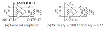
Figure \(\PageIndex{3}\): Amplifiers each with an input resistance \(R_{1}\) and output resistance \(R_{2}\).

The ‘\(2\)’ in the denominator arises because \(V_{1}\) and \(V_{2}\) are peak amplitudes of sinusoids in RF engineering. Thus the power gain is

\[\label{eq:13}G=\frac{P_{\text{out}}}{P_{\text{in}}}=\frac{V_{2}^{2}2R_{1}}{V_{1}^{2}2R_{2}}=\frac{R_{1}}{R_{2}}A_{v}^{2} \]

The power gain depends on the input and output resistance ratio of the amplifiers and this is commonly used to realize significant power gain even if the voltage gain is quite small. If the input and output resistances of the amplifier are the same, then the power gain is just the voltage gain squared.

In handling this situation some authors have used the unit \(\text{dBV}\) (decibel as a voltage ratio). This should not be used, decibels should always refer to a power ratio, and it is needlessly confusing to use \(\text{dBV}\) in RF engineering.

Example \(\PageIndex{6}\): Voltage Gain to Power Gain

Figure \(\PageIndex{3}\)(b) is a differential amplifier with a \(200\:\Omega\) input resistance and \(5\:\Omega\) output resistance. If the voltage \(A_{v}\) is \(0.6\), what is the power gain of the amplifier in \(\text{dB}\)?

Solution

The input and output powers are

\[\label{eq:14}P_{\text{in}}=\frac{1}{2}V_{1}^{2}/R_{1}\quad\text{and}\quad P_{\text{out}}=\frac{1}{2}V_{2}^{2}/R_{2}=\frac{1}{2}\frac{(A_{v}V_{1})^{2}}{R_{2}} \]

Thus the power gain is

\[\label{eq:15} G=\frac{P_{\text{out}}}{P_{\text{in}}}=\frac{(A_{v}V_{1})^{2}}{R_{2}}\left(\frac{V_{1}^{2}}{R_{1}}\right)^{-1}=\frac{R_{1}}{R_{2}}A_{v}^{2}=\frac{200}{5}0.6^{2}=14.4=11.58\text{ dB} \]

The surprising result is that even with a voltage gain of less than \(1\), a significant power gain can be obtained if the input and output resistances are different. A result used in many RF amplifiers.

Footnotes

[1] Named to honor Alexander Graham Bell, a prolific inventor and major contributor to RF communications.