
4.2: THE ROUTH CRITERION
- Page ID
- 58446
\( \newcommand{\vecs}[1]{\overset { \scriptstyle \rightharpoonup} {\mathbf{#1}} } \)
\( \newcommand{\vecd}[1]{\overset{-\!-\!\rightharpoonup}{\vphantom{a}\smash {#1}}} \)
\( \newcommand{\dsum}{\displaystyle\sum\limits} \)
\( \newcommand{\dint}{\displaystyle\int\limits} \)
\( \newcommand{\dlim}{\displaystyle\lim\limits} \)
\( \newcommand{\id}{\mathrm{id}}\) \( \newcommand{\Span}{\mathrm{span}}\)
( \newcommand{\kernel}{\mathrm{null}\,}\) \( \newcommand{\range}{\mathrm{range}\,}\)
\( \newcommand{\RealPart}{\mathrm{Re}}\) \( \newcommand{\ImaginaryPart}{\mathrm{Im}}\)
\( \newcommand{\Argument}{\mathrm{Arg}}\) \( \newcommand{\norm}[1]{\| #1 \|}\)
\( \newcommand{\inner}[2]{\langle #1, #2 \rangle}\)
\( \newcommand{\Span}{\mathrm{span}}\)
\( \newcommand{\id}{\mathrm{id}}\)
\( \newcommand{\Span}{\mathrm{span}}\)
\( \newcommand{\kernel}{\mathrm{null}\,}\)
\( \newcommand{\range}{\mathrm{range}\,}\)
\( \newcommand{\RealPart}{\mathrm{Re}}\)
\( \newcommand{\ImaginaryPart}{\mathrm{Im}}\)
\( \newcommand{\Argument}{\mathrm{Arg}}\)
\( \newcommand{\norm}[1]{\| #1 \|}\)
\( \newcommand{\inner}[2]{\langle #1, #2 \rangle}\)
\( \newcommand{\Span}{\mathrm{span}}\) \( \newcommand{\AA}{\unicode[.8,0]{x212B}}\)
\( \newcommand{\vectorA}[1]{\vec{#1}} % arrow\)
\( \newcommand{\vectorAt}[1]{\vec{\text{#1}}} % arrow\)
\( \newcommand{\vectorB}[1]{\overset { \scriptstyle \rightharpoonup} {\mathbf{#1}} } \)
\( \newcommand{\vectorC}[1]{\textbf{#1}} \)
\( \newcommand{\vectorD}[1]{\overrightarrow{#1}} \)
\( \newcommand{\vectorDt}[1]{\overrightarrow{\text{#1}}} \)
\( \newcommand{\vectE}[1]{\overset{-\!-\!\rightharpoonup}{\vphantom{a}\smash{\mathbf {#1}}}} \)
\( \newcommand{\vecs}[1]{\overset { \scriptstyle \rightharpoonup} {\mathbf{#1}} } \)
\(\newcommand{\longvect}{\overrightarrow}\)
\( \newcommand{\vecd}[1]{\overset{-\!-\!\rightharpoonup}{\vphantom{a}\smash {#1}}} \)
\(\newcommand{\avec}{\mathbf a}\) \(\newcommand{\bvec}{\mathbf b}\) \(\newcommand{\cvec}{\mathbf c}\) \(\newcommand{\dvec}{\mathbf d}\) \(\newcommand{\dtil}{\widetilde{\mathbf d}}\) \(\newcommand{\evec}{\mathbf e}\) \(\newcommand{\fvec}{\mathbf f}\) \(\newcommand{\nvec}{\mathbf n}\) \(\newcommand{\pvec}{\mathbf p}\) \(\newcommand{\qvec}{\mathbf q}\) \(\newcommand{\svec}{\mathbf s}\) \(\newcommand{\tvec}{\mathbf t}\) \(\newcommand{\uvec}{\mathbf u}\) \(\newcommand{\vvec}{\mathbf v}\) \(\newcommand{\wvec}{\mathbf w}\) \(\newcommand{\xvec}{\mathbf x}\) \(\newcommand{\yvec}{\mathbf y}\) \(\newcommand{\zvec}{\mathbf z}\) \(\newcommand{\rvec}{\mathbf r}\) \(\newcommand{\mvec}{\mathbf m}\) \(\newcommand{\zerovec}{\mathbf 0}\) \(\newcommand{\onevec}{\mathbf 1}\) \(\newcommand{\real}{\mathbb R}\) \(\newcommand{\twovec}[2]{\left[\begin{array}{r}#1 \\ #2 \end{array}\right]}\) \(\newcommand{\ctwovec}[2]{\left[\begin{array}{c}#1 \\ #2 \end{array}\right]}\) \(\newcommand{\threevec}[3]{\left[\begin{array}{r}#1 \\ #2 \\ #3 \end{array}\right]}\) \(\newcommand{\cthreevec}[3]{\left[\begin{array}{c}#1 \\ #2 \\ #3 \end{array}\right]}\) \(\newcommand{\fourvec}[4]{\left[\begin{array}{r}#1 \\ #2 \\ #3 \\ #4 \end{array}\right]}\) \(\newcommand{\cfourvec}[4]{\left[\begin{array}{c}#1 \\ #2 \\ #3 \\ #4 \end{array}\right]}\) \(\newcommand{\fivevec}[5]{\left[\begin{array}{r}#1 \\ #2 \\ #3 \\ #4 \\ #5 \\ \end{array}\right]}\) \(\newcommand{\cfivevec}[5]{\left[\begin{array}{c}#1 \\ #2 \\ #3 \\ #4 \\ #5 \\ \end{array}\right]}\) \(\newcommand{\mattwo}[4]{\left[\begin{array}{rr}#1 \amp #2 \\ #3 \amp #4 \\ \end{array}\right]}\) \(\newcommand{\laspan}[1]{\text{Span}\{#1\}}\) \(\newcommand{\bcal}{\cal B}\) \(\newcommand{\ccal}{\cal C}\) \(\newcommand{\scal}{\cal S}\) \(\newcommand{\wcal}{\cal W}\) \(\newcommand{\ecal}{\cal E}\) \(\newcommand{\coords}[2]{\left\{#1\right\}_{#2}}\) \(\newcommand{\gray}[1]{\color{gray}{#1}}\) \(\newcommand{\lgray}[1]{\color{lightgray}{#1}}\) \(\newcommand{\rank}{\operatorname{rank}}\) \(\newcommand{\row}{\text{Row}}\) \(\newcommand{\col}{\text{Col}}\) \(\renewcommand{\row}{\text{Row}}\) \(\newcommand{\nul}{\text{Nul}}\) \(\newcommand{\var}{\text{Var}}\) \(\newcommand{\corr}{\text{corr}}\) \(\newcommand{\len}[1]{\left|#1\right|}\) \(\newcommand{\bbar}{\overline{\bvec}}\) \(\newcommand{\bhat}{\widehat{\bvec}}\) \(\newcommand{\bperp}{\bvec^\perp}\) \(\newcommand{\xhat}{\widehat{\xvec}}\) \(\newcommand{\vhat}{\widehat{\vvec}}\) \(\newcommand{\uhat}{\widehat{\uvec}}\) \(\newcommand{\what}{\widehat{\wvec}}\) \(\newcommand{\Sighat}{\widehat{\Sigma}}\) \(\newcommand{\lt}{<}\) \(\newcommand{\gt}{>}\) \(\newcommand{\amp}{&}\) \(\definecolor{fillinmathshade}{gray}{0.9}\)The Routh test is a mathematical method that can be used to determine the number of zeros of a polynomial with positive real parts. If the test is applied to the denominator polynomial of a transfer function (also called the characteristic equation) the absence of any right-half-plane zeros of the characteristic equation guarantees system stability. One computational advantage of the Routh test is that it is not necessary to factor the polynomial to apply the test.
Evaluation of Stability
The test is described for a polynomial of the form
\[P(s) = a_0 s^n + a_1 s^{n - 1} + \cdots + a_{n - 1} s + a_n \label{eq4.2.1} \]
A necessary but not sufficient condition for all the zeros of Equation \(\ref{eq4.2.1}\) to have negative real parts is that all the \(a\)'s be present and that they all have the same sign. If this necessary condition is satisfied, an array of numbers is generated from the a's as follows. (This example is for \(n\) even. For \(n\) odd, \(a_n\) terminates the second row.)
\[\begin{array} {ccccccc} {a_0} & {a_2} & {a_4} & \cdot & \cdot & {a_{n - 2}} & {a_n} \\ {a_1} & {a_3} & {a_5} & \cdot & \cdot & {a_{n - 1}} & {0} \\ {\dfrac{a_1 a_2 - a_0 a_3}{a_1} = b_1} & {\dfrac{a_1 a_4 - a_0 a_5}{a_1} = b_2} & {\cdot} & \cdot & \cdot & {\dfrac{a_1 a_n - a_0 \cdot 0}{a_1} = b_{n/2}} & {0} \\ {\dfrac{b_1 a_3 - a_1 b_2}{b_1} = c_1} & {\dfrac{b_1 a_5 - a_1 b_3}{b_1} = c_2} & {\cdot} & \cdot & \cdot & {0} & {0} \\ {\dfrac{c_1 b_2 - b_1 c_2}{c_1} = d_1} & {\cdot} & {\cdot} & \cdot & \cdot & {0} & {0} \\ {\cdot} & {\cdot} & {\cdot} & \cdot & \cdot & {\cdot} & {\cdot} \\ {\cdot} & {\cdot} & {\cdot} & \cdot & \cdot & {\cdot} & {\cdot} \\ {0} & {0} & {\cdot} & \cdot & \cdot & {0} & {0} \end{array} \nonumber \]
As the array develops, progressively more elements of each row become zero, until only the first element of the \(n + 1\) row is nonzero. The total number of sign changes in the first column is then equal to the number of zeros of the original polynomial that lie in the right-half plane.
The use of the Routh criterion is illustrated using the polynomial
\[P(s) = s^4 + 9s^3 + 14s^2 + 266s + 260\label{eq4.2.3} \]
Since all coefficients are real and positive, the necessary condition for all roots of Equation \(\ref{eq4.2.3}\) to have negative real parts is satisfied. The array is
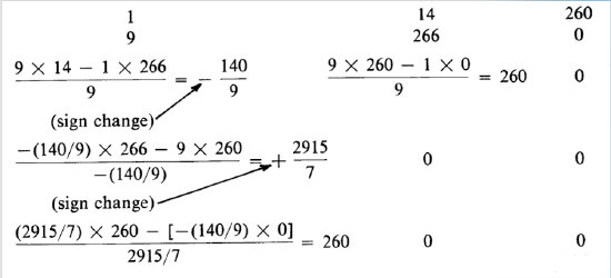
The two sign changes in the first column indicate two right-half-plane zeros. This result can be verified by factoring the original polynomial, showing that
\[s^4 + 9s^3 + 14s^2 + 266s + 260 = (s - 1 + j5)(s - 1 - j5) (s + 1)(s + 10) \nonumber \]
A second example is provided by the polynomial
\[P(s) = s^4 + 13s^2 + 58 s^2 + 306 s+ 260 \nonumber \]
The corresponding array is
\[\begin{array} {ccc} {1} & {58} & {260} \\ {13} & {306} & {0} \\ {\dfrac{13 \times 58 - 1 \times 306}{13} = \dfrac{448}{13}} & {\dfrac{13 \times 260 - 1 \times 0}{13} = 260} & {0} \\ {\dfrac{(448/13) \times 306 - 13 \times 260}{448/13} = \dfrac{23287}{112}} & {0} & {0} \\ {\dfrac{(23287/112) \times 260 - (448/13) \times 0}{23287/112} = 260} & {0} & {0} \end{array} \nonumber \]
Factoring verifies the result that there are no right-half-plane zeros for this polynomial, since
\[s^4 + 13s^3 + 58 s^2 + 306 s + 260 = (s + 1 + j5)(s + 1 - j5) (s + 1)(s + 10) \nonumber \]
Two kinds of difficulties can occur when applying the Routh test. It is possible that the first element in one row of the array is zero. In this case, the original polynomial is multiplied by \(s + \alpha\), where a is any positive real number, and the test is repeated. This procedure is illustrated using the polynomial
\[P(s) = s^5 + s^4 + 10s^3 + 10s^2 + 20s + 5 \label{eq4.2.8} \]
The first element of the third row of the array is zero.
\[\begin{array} {ccc} {1} & {10} & {20} \\ {1} & {10} & {5} \\ {0} & {15} & {0} \end{array} \nonumber \]
The difficulty is resolved by multiplying Equation \(\ref{eq4.2.8}\) by \(s + 1\), yielding
\[P'(s) = s^6 + 2s^5 + 11 s^4 + 20 s^3 + 30 s^2 + 25s + 5 \label{eq4.2.10} \]
The array for Equation \(\ref{eq4.2.10}\) is
\[\begin{array} {cccc} {1} & {11} & {30} & {5} \\ {2} & {20} & {25} & {0} \\ {1} & {17.5} & {5} & {0} \\ {-15} & {15} & {0} & {0} \\ {-18.5} & {5} & {0} & {0} \\ {10.95} & {0} & {0} & {0} \\ {5} & {0} & {0} & {0} \end{array}\label{eq4.2.11} \]
Since multiplication by \(s + 1\) did not add any right-half-plane zeros to Equation \(\ref{eq4.2.8}\), we conclude that the two right-half-plane zeros indicated by the array of Equation \(\ref{eq4.2.11}\) must be contained in the original polynomial.
The second possibility is that an entire row becomes zero. This condition indicates that there is a pair of roots on the imaginary axis, a pair of real roots located symmetrically with respect to the origin, or both kinds of pairs in the original polynomial. The terms in the row above the all-zero row are used as coefficients of an equation in even powers of \(s\) called the auxiliary equation. The zeros of this equation are the pairs mentioned above. The auxiliary equation can be differentiated with respect to \(s\), and the resultant coefficients are used in place of the all-zero row to continue the array. This type of difficulty is illustrated with the polynomial
\[P(s) = s^4 + 11s^3 + 11s^2 + 11s + 10 = (s + j)(s - j) (s + 1) (s + 10)\label{eq4.2.12} \]
The array is
\[\begin{array} {ccc} {1} & {11} & {10} \\ {11} & {11} & {0} \\ {10} & {10} & {0} \\ {0} & {0} & {0} \end{array}\label{eq4.2.13} \]
The auxiliary equation is
\[Q(s) = 10s^2 + 10\label{eq4.2.14} \]
The roots of the equation are the two imaginary zeros of Equation \(\ref{eq4.2.12}\). Differentiating Equation \(\ref{eq4.2.14}\) and using the nonzero coefficient to replace the first element of row 4 of Equation \(\ref{eq4.2.13}\) yields a new array.
\[\begin{array} {ccc} {1} & {11} & {10} \\ {11} & {11} & {0} \\ {10} & {10} & {0} \\ {20} & {0} & {0} \\ {10} & {0} & {0} \end{array} \nonumber \]
The absence of sign changes in the array verifies that the original poly nomial has no zeros in the right-half plane.
Note that, while there are no closed-loop poles in the right-half plane, a system with a characteristic equation given by Equation \(\ref{eq4.2.12}\) is unstable by our definition since it has a pair of poles on the imaginary axis. Examining only the left-hand column of the Routh array only identifies the number of right-half-plane zeros of the tested polynomial. Imaginary-axis zeros can be found by the manipulations involving the auxiliary equation.
Design Aid
The Routh criterion is most frequently used to determine the stability of a feedback system. In certain cases, however, more quantitative design information is obtainable, as illustrated by the following examples.
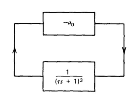
A phase-shift oscillator can be constructed by applying sufficient negative feedback around a network that has three or more poles. If an amplifier with frequency-independent gain is combined with a network with three coincident poles, the block diagram for the resultant system is as shown in Figure 4.2. The value of \(a_0\) necessary to sustain oscillations can be determined by Routh analysis.(The Routh test applied to this example offers computational advantages compared to the direct factoring used for a similar transfer function in the example of Section 4.1.)
Stability investigations for Figure 4.2 are complicated by the fact that the
oscillator has no input; thus we cannot use the poles of an input-to-output transfer function to determine stability. We should note that the stability of a linear system is a property of the system itself and is thus independent of input signals that may be applied to it. Any unstable physical system will demonstrate its instability with no input, since runaway behavior will be stimulated by always present noise. Even in a purely mathematical linear system, stability is determined by the location of the closed-loop poles, and these locations are clearly input independent.
The analysis of the oscillator is initiated by recalling that the characteristic equation of any feedback system is one minus its loop transmission. Therefore
\[P(s) = 1 + \dfrac{a_0}{(\tau s + 1)^3} \nonumber \]
In this and other calculations involving the characteristic equation, it is possible to clear fractions since the location of the zeros are not altered by this operation. After clearing fractions and identifying coefficients, the Routh array is
\[\begin{array} {cc} {\tau^3} & {3 \tau} \\ {3 \tau^2} & {1 + a_0} \\ {\dfrac{(8 - a_0) \tau}{3}} & {0} \\ {1 + a_0} & {0} \end{array} \nonumber \]
Assuming \(\tau\) is positive, roots with positive real parts occur for \(a_0 < -1\) (one right-half-plane zero) and for \(a_0 > +8\) (two right-half-plane zeros).
Laplace analysis indicates that generation of a constant-amplitude sinusoidal oscillation requires a pole pair on the imaginary axis. In practice, a complex pole pair is located slightly to the right of the imaginary axis. An intentionally introduced nonlinearity can then be used to limit the amplitude of the oscillation (see Section 6.3.3). Thus, a practical oscillator circuit is obtained with \(a_0 > 8\).
The frequency of oscillation with \(a_0 = 8\) can be determined by examining the array with this value for \(a_0\). Under these conditions the third row becomes all zero. The auxiliary equation is
\[Q(s) = 3\tau^2 s^2 + 9 \nonumber \]
and the equation has zeros at \(s = \pm j \sqrt{3}/\tau\), indicating oscillation at \(\sqrt{3}/\tau\) radians per second for \(a_0 = 8\).
As a second example of the type of design information that can be obtained via Routh analysis, consider an operational amplifier with an open-loop transfer function
\[a(s) = \dfrac{a_0}{(s + 1) (10^{-6} s + 1) (10^{-7} s + 1)} \nonumber \]
It is assumed that this amplifier is connected as a unity-gain noninverting amplifier, and we wish to determine the range of values of ao for which all closed-loop poles have real parts more negative than \(-2 \times 10^5 \text{sec}^{-1}\). This condition on closed-loop pole location implies that any pulse response of the system will decay at least as fast as \(K e^{-2 \times 10^5 t}\) after the exciting pulse returns to zero. The constant \(K\) is dependent on conditions at the time the input becomes zero.
The characteristic equation for the amplifier is (after dropping insignificant terms)
\[P(s) = 10^{-13} s^3 + 1.1 \times 10^{-6} s^2 + s + 1 + a_0 \label{eq4.2.20} \]
In order to determine the range of ao for which all zeros of this characteristic equation have real parts more negative than \(-2 \times 10^5 \text{sec}^{-1}\), it is only necessary to make a change of variable in Equation \(\ref{eq4.2.20}\) and apply Routh's criterion to the modified equation. In particular, application of the Routh test to a polynomial obtained by substituting
\[\lambda = s + c \nonumber \]
will determine the number of zeros of the original polynomial with real parts more positive than \(-c\), since this substitution shifts singularities in the \(s\) plane to the right by an amount \(c\) as they are mapped into the \(\lambda\) plane. If the indicated substitution is made with \(c = 2 \times 10^5 \text{sec}^{-1}\), Equation \(\ref{eq4.2.20}\) becomes
\[P(\lambda) = 10^{-13} \lambda^3 + 10^{-6} \lambda^2 + 0.57 \lambda - 1.57 \times 10^5 + a_0 \nonumber \]
The Routh array is
\[\begin{array} {cc} {10^{-13}} & {0.57} \\ {10^{-6}} & {-1.57 \times 10^5 + a_0} \\ {0.59 - 10^{-7} a_0} & {0} \\ {-1.57 \times 10^5 + a_0} & {0} \end{array} \nonumber \]
This array shows that Eqn \(\ref{eq4.2.20}\) has one zero with a real part more positive than \(-2 \times 10^5 \text{sec}^{-1}\) for \(a_0 < 1.57 \times 10^5\), and has two zeros to the right of the dividing line for \(a_0 > 5.9 \times 10^6\). Accordingly, all zeros have real parts more negative than \(-2 \times 10^5 \text{sec}^{-1}\) only for
\[1.57 \times 10^5 < a_0 < 5.9 \times 10^6 \nonumber \]