Engineering LibreTexts

3.3: Beating between Tones

  • Page ID
    9963
  • \( \newcommand{\vecs}[1]{\overset { \scriptstyle \rightharpoonup} {\mathbf{#1}} } \)

    \( \newcommand{\vecd}[1]{\overset{-\!-\!\rightharpoonup}{\vphantom{a}\smash {#1}}} \)

    \( \newcommand{\id}{\mathrm{id}}\) \( \newcommand{\Span}{\mathrm{span}}\)

    ( \newcommand{\kernel}{\mathrm{null}\,}\) \( \newcommand{\range}{\mathrm{range}\,}\)

    \( \newcommand{\RealPart}{\mathrm{Re}}\) \( \newcommand{\ImaginaryPart}{\mathrm{Im}}\)

    \( \newcommand{\Argument}{\mathrm{Arg}}\) \( \newcommand{\norm}[1]{\| #1 \|}\)

    \( \newcommand{\inner}[2]{\langle #1, #2 \rangle}\)

    \( \newcommand{\Span}{\mathrm{span}}\)

    \( \newcommand{\id}{\mathrm{id}}\)

    \( \newcommand{\Span}{\mathrm{span}}\)

    \( \newcommand{\kernel}{\mathrm{null}\,}\)

    \( \newcommand{\range}{\mathrm{range}\,}\)

    \( \newcommand{\RealPart}{\mathrm{Re}}\)

    \( \newcommand{\ImaginaryPart}{\mathrm{Im}}\)

    \( \newcommand{\Argument}{\mathrm{Arg}}\)

    \( \newcommand{\norm}[1]{\| #1 \|}\)

    \( \newcommand{\inner}[2]{\langle #1, #2 \rangle}\)

    \( \newcommand{\Span}{\mathrm{span}}\) \( \newcommand{\AA}{\unicode[.8,0]{x212B}}\)

    \( \newcommand{\vectorA}[1]{\vec{#1}}      % arrow\)

    \( \newcommand{\vectorAt}[1]{\vec{\text{#1}}}      % arrow\)

    \( \newcommand{\vectorB}[1]{\overset { \scriptstyle \rightharpoonup} {\mathbf{#1}} } \)

    \( \newcommand{\vectorC}[1]{\textbf{#1}} \)

    \( \newcommand{\vectorD}[1]{\overrightarrow{#1}} \)

    \( \newcommand{\vectorDt}[1]{\overrightarrow{\text{#1}}} \)

    \( \newcommand{\vectE}[1]{\overset{-\!-\!\rightharpoonup}{\vphantom{a}\smash{\mathbf {#1}}}} \)

    \( \newcommand{\vecs}[1]{\overset { \scriptstyle \rightharpoonup} {\mathbf{#1}} } \)

    \( \newcommand{\vecd}[1]{\overset{-\!-\!\rightharpoonup}{\vphantom{a}\smash {#1}}} \)

    \(\newcommand{\avec}{\mathbf a}\) \(\newcommand{\bvec}{\mathbf b}\) \(\newcommand{\cvec}{\mathbf c}\) \(\newcommand{\dvec}{\mathbf d}\) \(\newcommand{\dtil}{\widetilde{\mathbf d}}\) \(\newcommand{\evec}{\mathbf e}\) \(\newcommand{\fvec}{\mathbf f}\) \(\newcommand{\nvec}{\mathbf n}\) \(\newcommand{\pvec}{\mathbf p}\) \(\newcommand{\qvec}{\mathbf q}\) \(\newcommand{\svec}{\mathbf s}\) \(\newcommand{\tvec}{\mathbf t}\) \(\newcommand{\uvec}{\mathbf u}\) \(\newcommand{\vvec}{\mathbf v}\) \(\newcommand{\wvec}{\mathbf w}\) \(\newcommand{\xvec}{\mathbf x}\) \(\newcommand{\yvec}{\mathbf y}\) \(\newcommand{\zvec}{\mathbf z}\) \(\newcommand{\rvec}{\mathbf r}\) \(\newcommand{\mvec}{\mathbf m}\) \(\newcommand{\zerovec}{\mathbf 0}\) \(\newcommand{\onevec}{\mathbf 1}\) \(\newcommand{\real}{\mathbb R}\) \(\newcommand{\twovec}[2]{\left[\begin{array}{r}#1 \\ #2 \end{array}\right]}\) \(\newcommand{\ctwovec}[2]{\left[\begin{array}{c}#1 \\ #2 \end{array}\right]}\) \(\newcommand{\threevec}[3]{\left[\begin{array}{r}#1 \\ #2 \\ #3 \end{array}\right]}\) \(\newcommand{\cthreevec}[3]{\left[\begin{array}{c}#1 \\ #2 \\ #3 \end{array}\right]}\) \(\newcommand{\fourvec}[4]{\left[\begin{array}{r}#1 \\ #2 \\ #3 \\ #4 \end{array}\right]}\) \(\newcommand{\cfourvec}[4]{\left[\begin{array}{c}#1 \\ #2 \\ #3 \\ #4 \end{array}\right]}\) \(\newcommand{\fivevec}[5]{\left[\begin{array}{r}#1 \\ #2 \\ #3 \\ #4 \\ #5 \\ \end{array}\right]}\) \(\newcommand{\cfivevec}[5]{\left[\begin{array}{c}#1 \\ #2 \\ #3 \\ #4 \\ #5 \\ \end{array}\right]}\) \(\newcommand{\mattwo}[4]{\left[\begin{array}{rr}#1 \amp #2 \\ #3 \amp #4 \\ \end{array}\right]}\) \(\newcommand{\laspan}[1]{\text{Span}\{#1\}}\) \(\newcommand{\bcal}{\cal B}\) \(\newcommand{\ccal}{\cal C}\) \(\newcommand{\scal}{\cal S}\) \(\newcommand{\wcal}{\cal W}\) \(\newcommand{\ecal}{\cal E}\) \(\newcommand{\coords}[2]{\left\{#1\right\}_{#2}}\) \(\newcommand{\gray}[1]{\color{gray}{#1}}\) \(\newcommand{\lgray}[1]{\color{lightgray}{#1}}\) \(\newcommand{\rank}{\operatorname{rank}}\) \(\newcommand{\row}{\text{Row}}\) \(\newcommand{\col}{\text{Col}}\) \(\renewcommand{\row}{\text{Row}}\) \(\newcommand{\nul}{\text{Nul}}\) \(\newcommand{\var}{\text{Var}}\) \(\newcommand{\corr}{\text{corr}}\) \(\newcommand{\len}[1]{\left|#1\right|}\) \(\newcommand{\bbar}{\overline{\bvec}}\) \(\newcommand{\bhat}{\widehat{\bvec}}\) \(\newcommand{\bperp}{\bvec^\perp}\) \(\newcommand{\xhat}{\widehat{\xvec}}\) \(\newcommand{\vhat}{\widehat{\vvec}}\) \(\newcommand{\uhat}{\widehat{\uvec}}\) \(\newcommand{\what}{\widehat{\wvec}}\) \(\newcommand{\Sighat}{\widehat{\Sigma}}\) \(\newcommand{\lt}{<}\) \(\newcommand{\gt}{>}\) \(\newcommand{\amp}{&}\) \(\definecolor{fillinmathshade}{gray}{0.9}\)

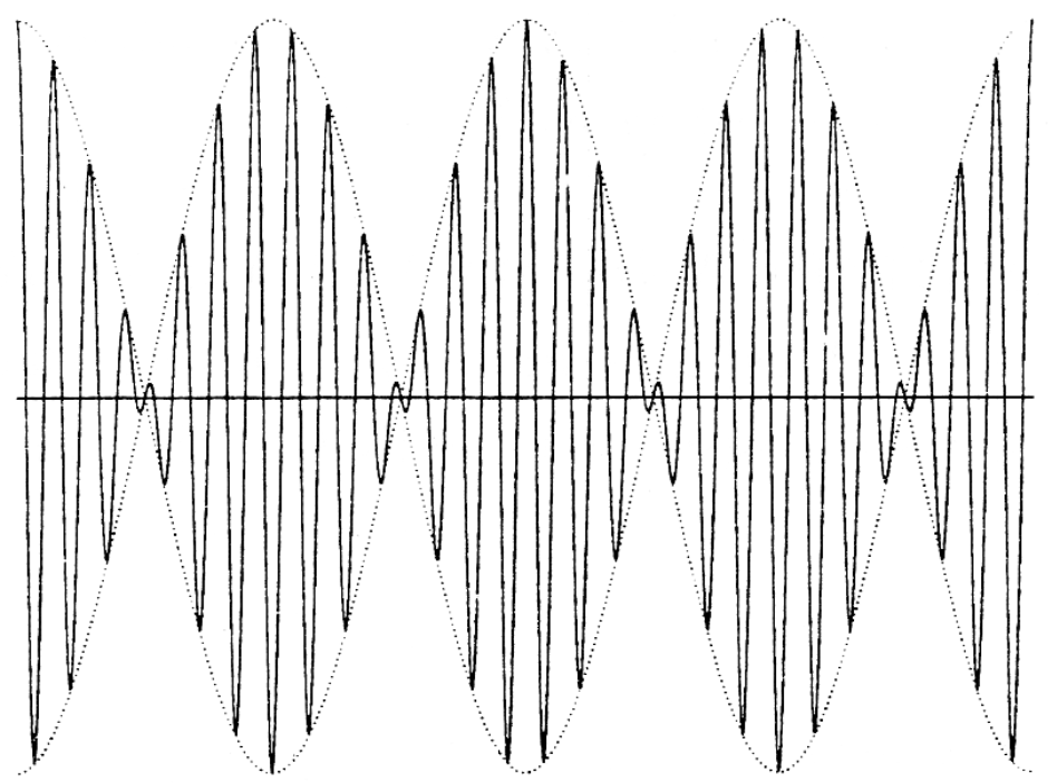
    Perhaps you have heard two slightly mistuned musical instruments play pure tones whose frequencies are close but not equal. If so, you have sensed a beating phenomenon wherein a pure tone seems to wax and wane. This waxing and waning tone is, in fact, a tone whose frequency is the average of the two mismatched frequencies, amplitude modulated by a tone whose “beat” frequency is half the difference between the two mismatched frequencies. The effect is illustrated in the Figure. Let's see if we can derive a mathematical model for the beating of tones.

    We begin with two pure tones whose frequencies are \(ω_0+ν\) and \(ω_0−ν\) (for example, \(ω_0=2π×10^3\mathrm{rad}/\mathrm{sec}\) and \(ν=2π \mathrm{rad}/\mathrm{sec}\)). The average frequency is \(ω_0\), and the difference frequency is \(2ν\). What you hear is the sum of the two tones:

    \[x(t)=A_1\cos[(ω_0+ν)t+φ_1]+A_2\cos[(ω_0−ν)t+φ_2] \nonumber \]

    The first tone has amplitude \(A_1\) and phase \(φ_1\); the second has amplitude \(A_2\) and phase \(φ_2\). We will assume that the two amplitudes are equal to \(A\). Furthermore, whatever the phases, we may write them as

    \[φ_1=φ+ψ;\mathrm{and};φ_2=φ−ψ \nonumber \]

    \[φ=\frac 1 2 (φ_1+φ_2);\mathrm{and}ψ=\frac 1 2 (φ_1−φ_2) \nonumber \]

    BeatBetweenTones.PNG
    Beating between Tones

    Recall our trick for representing \(x(t)\) as a complex phasor:

    \[x(t)=A\mathrm{Re}\{e{j[(ω_0+ν)t+φ+ψ]},+,e^{j[(ω_0−ν)t+φ−ψ]}\} \nonumber \]

    \[=A\mathrm{Re}\{e^{j(ω_0t+φ)},[e^{j(νt+ψ)}+e^{−j(νt+ψ)]}\} \nonumber \]

    \[=2A\mathrm{Re}\{e^{j(ω_0t+φ)},\cos(νt+ψ)\} \nonumber \]

    \[=2A\cos(ω_0t+φ)\cos(νt+ψ) \nonumber \]

    This is an amplitude modulated wave, wherein a low frequency signal with beat frequency \(ν\) rad/sec modulates a high frequency signal with carrier frequency \(ω_0\) rad/sec. Over short periods of time, the modulating term \(\cos{νt+ψ}\) remains essentially constant while the carrier term \(\cos{ω_0t+φ}\) turns out many cycles of its tone. For example, if \(t\) runs from 0 to \(\frac {2π} {10ν}\) (about 0.1 seconds in our example), then the modulating wave turns out just 1/10 cycle while the carrier turns out \(10νω_Δ\) cycles (about 100 in our example). Every time \(νt\) changes by \(2π\) radians, then the modulating term goes from a maximum (a wax) through a minimum (a wane) and back to a maximum. This cycle takes

    \[νt=2π⇔t=\frac {2π} {ν} \mathrm{seconds} \nonumber \]

    which is 1 second in our example. In this 1 second the carrier turns out 1000 cycles.

    Exercise \(\PageIndex{1}\)

    Find out the frequency of A above middle C on a piano. Assume two pianos are mistuned by \(±1\mathrm{Hz}(±2π/mathrm{rad/sec})\). Find their beat frequency \(ν\) and their carrier frequency \(ω_0\).

    Exercise \(\PageIndex{2}\)

    (MATLAB) Write a MATLAB program to compute and plot

    \(A\cos[(ω_0+ν)t+φ_1],A\cos[(ω_0−ν)t+φ_2]\), and their sum. Then compute and plot \(2A\cos(ω_0t+φ)\cos(νt+ψ)\).

    Verify that the sum equals this latter signal.


    This page titled 3.3: Beating between Tones is shared under a CC BY 3.0 license and was authored, remixed, and/or curated by Louis Scharf (OpenStax CNX) via source content that was edited to the style and standards of the LibreTexts platform.

    • Was this article helpful?