
3.4: Multiphase Power
- Page ID
- 9964

\( \newcommand{\vecs}[1]{\overset { \scriptstyle \rightharpoonup} {\mathbf{#1}} } \)
\( \newcommand{\vecd}[1]{\overset{-\!-\!\rightharpoonup}{\vphantom{a}\smash {#1}}} \)
\( \newcommand{\id}{\mathrm{id}}\) \( \newcommand{\Span}{\mathrm{span}}\)
( \newcommand{\kernel}{\mathrm{null}\,}\) \( \newcommand{\range}{\mathrm{range}\,}\)
\( \newcommand{\RealPart}{\mathrm{Re}}\) \( \newcommand{\ImaginaryPart}{\mathrm{Im}}\)
\( \newcommand{\Argument}{\mathrm{Arg}}\) \( \newcommand{\norm}[1]{\| #1 \|}\)
\( \newcommand{\inner}[2]{\langle #1, #2 \rangle}\)
\( \newcommand{\Span}{\mathrm{span}}\)
\( \newcommand{\id}{\mathrm{id}}\)
\( \newcommand{\Span}{\mathrm{span}}\)
\( \newcommand{\kernel}{\mathrm{null}\,}\)
\( \newcommand{\range}{\mathrm{range}\,}\)
\( \newcommand{\RealPart}{\mathrm{Re}}\)
\( \newcommand{\ImaginaryPart}{\mathrm{Im}}\)
\( \newcommand{\Argument}{\mathrm{Arg}}\)
\( \newcommand{\norm}[1]{\| #1 \|}\)
\( \newcommand{\inner}[2]{\langle #1, #2 \rangle}\)
\( \newcommand{\Span}{\mathrm{span}}\) \( \newcommand{\AA}{\unicode[.8,0]{x212B}}\)
\( \newcommand{\vectorA}[1]{\vec{#1}} % arrow\)
\( \newcommand{\vectorAt}[1]{\vec{\text{#1}}} % arrow\)
\( \newcommand{\vectorB}[1]{\overset { \scriptstyle \rightharpoonup} {\mathbf{#1}} } \)
\( \newcommand{\vectorC}[1]{\textbf{#1}} \)
\( \newcommand{\vectorD}[1]{\overrightarrow{#1}} \)
\( \newcommand{\vectorDt}[1]{\overrightarrow{\text{#1}}} \)
\( \newcommand{\vectE}[1]{\overset{-\!-\!\rightharpoonup}{\vphantom{a}\smash{\mathbf {#1}}}} \)
\( \newcommand{\vecs}[1]{\overset { \scriptstyle \rightharpoonup} {\mathbf{#1}} } \)
\( \newcommand{\vecd}[1]{\overset{-\!-\!\rightharpoonup}{\vphantom{a}\smash {#1}}} \)
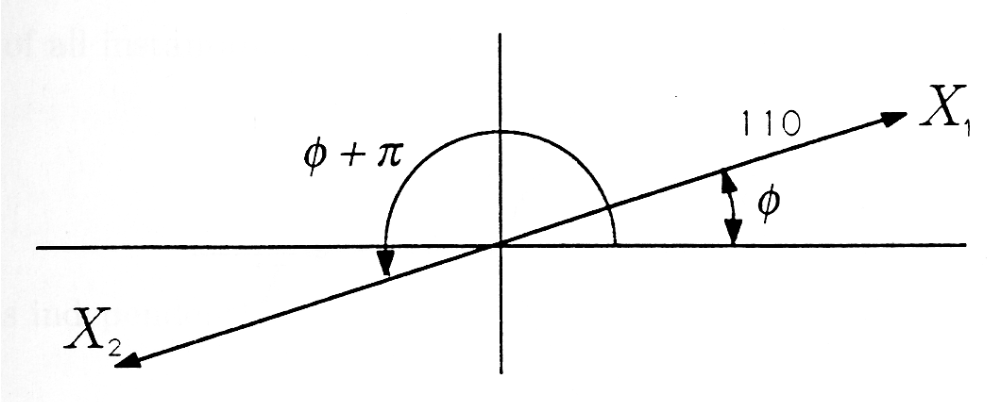
\(\newcommand{\avec}{\mathbf a}\) \(\newcommand{\bvec}{\mathbf b}\) \(\newcommand{\cvec}{\mathbf c}\) \(\newcommand{\dvec}{\mathbf d}\) \(\newcommand{\dtil}{\widetilde{\mathbf d}}\) \(\newcommand{\evec}{\mathbf e}\) \(\newcommand{\fvec}{\mathbf f}\) \(\newcommand{\nvec}{\mathbf n}\) \(\newcommand{\pvec}{\mathbf p}\) \(\newcommand{\qvec}{\mathbf q}\) \(\newcommand{\svec}{\mathbf s}\) \(\newcommand{\tvec}{\mathbf t}\) \(\newcommand{\uvec}{\mathbf u}\) \(\newcommand{\vvec}{\mathbf v}\) \(\newcommand{\wvec}{\mathbf w}\) \(\newcommand{\xvec}{\mathbf x}\) \(\newcommand{\yvec}{\mathbf y}\) \(\newcommand{\zvec}{\mathbf z}\) \(\newcommand{\rvec}{\mathbf r}\) \(\newcommand{\mvec}{\mathbf m}\) \(\newcommand{\zerovec}{\mathbf 0}\) \(\newcommand{\onevec}{\mathbf 1}\) \(\newcommand{\real}{\mathbb R}\) \(\newcommand{\twovec}[2]{\left[\begin{array}{r}#1 \\ #2 \end{array}\right]}\) \(\newcommand{\ctwovec}[2]{\left[\begin{array}{c}#1 \\ #2 \end{array}\right]}\) \(\newcommand{\threevec}[3]{\left[\begin{array}{r}#1 \\ #2 \\ #3 \end{array}\right]}\) \(\newcommand{\cthreevec}[3]{\left[\begin{array}{c}#1 \\ #2 \\ #3 \end{array}\right]}\) \(\newcommand{\fourvec}[4]{\left[\begin{array}{r}#1 \\ #2 \\ #3 \\ #4 \end{array}\right]}\) \(\newcommand{\cfourvec}[4]{\left[\begin{array}{c}#1 \\ #2 \\ #3 \\ #4 \end{array}\right]}\) \(\newcommand{\fivevec}[5]{\left[\begin{array}{r}#1 \\ #2 \\ #3 \\ #4 \\ #5 \\ \end{array}\right]}\) \(\newcommand{\cfivevec}[5]{\left[\begin{array}{c}#1 \\ #2 \\ #3 \\ #4 \\ #5 \\ \end{array}\right]}\) \(\newcommand{\mattwo}[4]{\left[\begin{array}{rr}#1 \amp #2 \\ #3 \amp #4 \\ \end{array}\right]}\) \(\newcommand{\laspan}[1]{\text{Span}\{#1\}}\) \(\newcommand{\bcal}{\cal B}\) \(\newcommand{\ccal}{\cal C}\) \(\newcommand{\scal}{\cal S}\) \(\newcommand{\wcal}{\cal W}\) \(\newcommand{\ecal}{\cal E}\) \(\newcommand{\coords}[2]{\left\{#1\right\}_{#2}}\) \(\newcommand{\gray}[1]{\color{gray}{#1}}\) \(\newcommand{\lgray}[1]{\color{lightgray}{#1}}\) \(\newcommand{\rank}{\operatorname{rank}}\) \(\newcommand{\row}{\text{Row}}\) \(\newcommand{\col}{\text{Col}}\) \(\renewcommand{\row}{\text{Row}}\) \(\newcommand{\nul}{\text{Nul}}\) \(\newcommand{\var}{\text{Var}}\) \(\newcommand{\corr}{\text{corr}}\) \(\newcommand{\len}[1]{\left|#1\right|}\) \(\newcommand{\bbar}{\overline{\bvec}}\) \(\newcommand{\bhat}{\widehat{\bvec}}\) \(\newcommand{\bperp}{\bvec^\perp}\) \(\newcommand{\xhat}{\widehat{\xvec}}\) \(\newcommand{\vhat}{\widehat{\vvec}}\) \(\newcommand{\uhat}{\widehat{\uvec}}\) \(\newcommand{\what}{\widehat{\wvec}}\) \(\newcommand{\Sighat}{\widehat{\Sigma}}\) \(\newcommand{\lt}{<}\) \(\newcommand{\gt}{>}\) \(\newcommand{\amp}{&}\) \(\definecolor{fillinmathshade}{gray}{0.9}\)The electrical service to your home is a two-phase service.1 This means that two 110 volt, 60 Hz lines, plus neutral, terminate in the panel. The lines are π radians (180) out of phase, so we can write them as
\[ \begin{align*} x_1(t) &=110\cos[2π(60)t+φ] \\[4pt] &=\mathrm{Re}\{110e^{j[2π(60)t+φ]}\} \\[4pt] &=\mathrm{Re}\{X_1e^{j2π(60)t}\} \end{align*} \nonumber \]
\[X_1=110ej^{φ} \nonumber \]
\[ \begin{align*} x_2(t) &=110\cos[2π(60)t+φ+π] \\[4pt] &=\mathrm{Re}\{110e^{j[2π(60)t+φ+π]}\} \\[4pt] &=\mathrm{Re}\{X_2ej^{2π(60)t}\} \end{align*} \nonumber \]
\[X_2=110e^{j(φ+π)} \nonumber \]
These two voltages are illustrated as the phasors \(X_1\) and \(X_2\) in the Figure.
You may use \(x_1(t)\) to drive your clock radio or your toaster and the difference between \(x_1(t)\) and \(x_2(t)\) to drive your range or dryer:
\[x_1(t)−x_2(t)=220\cos[2π(60)t+φ] \nonumber \]
The phasor representation of this difference is
\[X_1−X_2=220e^{jφ} \nonumber \]
The breakers in a breaker box span the \(x_1\)−to-neutral bus for 110 volts and the \(x_1-\mathrm{to}-x_2\) buses for 220 volts.
Sketch the phasor \(X_1−X_2\) on the Figure.
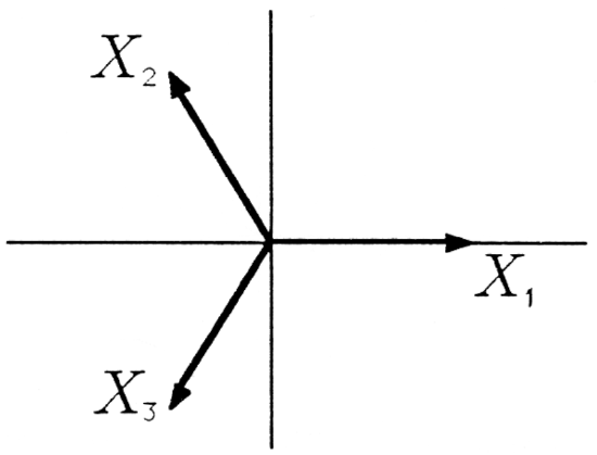
Most industrial installations use a three-phase service consisting of the signals \(x_1(t)\),\(x_2(t)\), and \(x_3(t)\):
\(x_n(t)=110\mathrm{Re}\{e^{j[ω_0t+n(2π/3)]}\}↔X_n=110e^{jn(2π/3)},n=1,2,3\)
The phasors for three-phase power are illustrated in the Figure.
Sketch the phasor \(X_2−X_1\) corresponding to \(x_2(t)−x_1(t)\) on Exercise. Compute the voltage you can get with \(x_2(t)−x_1(t)\). This answer explains why you do not get 220 volts in three-phase circuits. What do you get?
Constant Power
Two- and three-phase power generalizes in an obvious way to N-phase power. In such a scheme, the N signals \(x_n(n=0,1,...,N−1)\) are
\[ \begin{align*} x_n(t) &=A\cos(ωt+\frac {2π} {N} n) \\[4pt] &=\mathrm{Re}[Ae^{j2πn/N}e^{jωt}]↔X_n=Aej^{2πn/N} \end{align*} \nonumber \]
The phasors \(X_n\) are \(Ae^{j2π(n/N)}\). The sum of all \(N\) signals is zero:
\[\begin{align*} \sum^{N−1}_{n=0}x_n(t) &= \mathrm{Re}\{A∑^{N−1}_{n=0} e^{j2πn/N} e^{jωt} \} \\[4pt] &=\mathrm{Re}{A\frac {1−ej^{2π}} {1−e^{j2π/N}} e^{jωt}} \\[4pt] &=0 \end{align*} \nonumber \]
But what about the sum of the instantaneous powers? Define the instantaneous power of the nth signal to be
\[ \begin{align*} p_n(t) &=x^2_n(t) &=A^2\cos^2(ωt+\frac{2π}{N} n) \\[4pt] &=\frac {A^2}{2} + \frac{A^2}{ 2} \cos(2ωt + 2\frac {2π} {N} n) \\[4pt] &=\frac {A^2} {2} + \mathrm{Re}\{\frac {A^2} 2 e^{j(2π/N)2n} e^{j2ωt}\} \end{align*} \nonumber \]
The sum of all instantaneous powers is
\[P=\sum_{n=0}^{N−1}p_n(t) = N\frac {A^2} 2 \nonumber \]
and this is independent of time!
Carry out the computations of Equation 5.4.16 to prove that instantaneous power P is constant in the N-phase power scheme.
Footnotes
- It really is, although it is said to be “single phase” because of the way it is picked off a single phase of a primary source. You will hear more about this in circuits and power courses