6.1: Introduction
- Page ID
- 9982
\( \newcommand{\vecs}[1]{\overset { \scriptstyle \rightharpoonup} {\mathbf{#1}} } \)
\( \newcommand{\vecd}[1]{\overset{-\!-\!\rightharpoonup}{\vphantom{a}\smash {#1}}} \)
\( \newcommand{\id}{\mathrm{id}}\) \( \newcommand{\Span}{\mathrm{span}}\)
( \newcommand{\kernel}{\mathrm{null}\,}\) \( \newcommand{\range}{\mathrm{range}\,}\)
\( \newcommand{\RealPart}{\mathrm{Re}}\) \( \newcommand{\ImaginaryPart}{\mathrm{Im}}\)
\( \newcommand{\Argument}{\mathrm{Arg}}\) \( \newcommand{\norm}[1]{\| #1 \|}\)
\( \newcommand{\inner}[2]{\langle #1, #2 \rangle}\)
\( \newcommand{\Span}{\mathrm{span}}\)
\( \newcommand{\id}{\mathrm{id}}\)
\( \newcommand{\Span}{\mathrm{span}}\)
\( \newcommand{\kernel}{\mathrm{null}\,}\)
\( \newcommand{\range}{\mathrm{range}\,}\)
\( \newcommand{\RealPart}{\mathrm{Re}}\)
\( \newcommand{\ImaginaryPart}{\mathrm{Im}}\)
\( \newcommand{\Argument}{\mathrm{Arg}}\)
\( \newcommand{\norm}[1]{\| #1 \|}\)
\( \newcommand{\inner}[2]{\langle #1, #2 \rangle}\)
\( \newcommand{\Span}{\mathrm{span}}\) \( \newcommand{\AA}{\unicode[.8,0]{x212B}}\)
\( \newcommand{\vectorA}[1]{\vec{#1}} % arrow\)
\( \newcommand{\vectorAt}[1]{\vec{\text{#1}}} % arrow\)
\( \newcommand{\vectorB}[1]{\overset { \scriptstyle \rightharpoonup} {\mathbf{#1}} } \)
\( \newcommand{\vectorC}[1]{\textbf{#1}} \)
\( \newcommand{\vectorD}[1]{\overrightarrow{#1}} \)
\( \newcommand{\vectorDt}[1]{\overrightarrow{\text{#1}}} \)
\( \newcommand{\vectE}[1]{\overset{-\!-\!\rightharpoonup}{\vphantom{a}\smash{\mathbf {#1}}}} \)
\( \newcommand{\vecs}[1]{\overset { \scriptstyle \rightharpoonup} {\mathbf{#1}} } \)
\( \newcommand{\vecd}[1]{\overset{-\!-\!\rightharpoonup}{\vphantom{a}\smash {#1}}} \)
Notes to Teachers and Students:
Filtering is one of the most important things that electrical and computer engineers do. In this chapter we extend everyday understanding of filters to numerical filters. We then study weighted moving averages and exponential averages. We define the important test signals for electrical and computer engineering and show how filters respond to them. The idea that filters are characterized by their response to simple test signals is fundamental. In the numerical experiment, students explore the frequency response of a simple filter, a concept that forms the basis of circuit theory, electronics, optics and lasers, solid-state devices, communications, and control.
Introduction
A filter is any device that passes material, light, sound, current, velocity, or information according to some rule of selectivity. Material (or mechanical) filters are commonplace in your everyday life:
- coffee filters pass flavored water while filtering out coffee grounds;
- Goretex fibers pass small, warm perspiration droplets while filtering out large, cool droplets of rain or snow;
- fiberglass strands in a furnace filter pass warm air while filtering out particles of dirt and dust;
- a centrifuge retains material of low density while spinning out (or filtering out) material of high density; and
- an electrostatic precipitator filters out dust and other effluents by attaching charge to them and using an electric field to move the charged particles to a high potential drain.
The first three of these examples selectively pass material according to size; the last two selectively pass material according to its mass density.
Typical filters for light are
- UV filters on camera lenses and eyeglasses that pass light in the range of visible wavelengths while blocking light in the invisible (but damaging) ultraviolet range;
- polaroid lenses that pass light that is randomly polarized while blocking out glare that is linearly polarized;
- green fabrics that reflect green light and absorb other colors;
- red taillights that pass light in the long wavelength red range and reflect light in the short wavelength violet range (look at the inside of your taillights to see violet); and
- glacial ice that absorbs all but the blue wavelengths so that it appears blue.
List as many examples of natural and man-made sound filters as you can.
Satellite Television
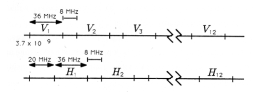
Among current filters, the tuner in a super-heterodyne receiver is, perhaps, the first example that comes to mind. But satellite TV filters are another fascinating example. A typical C-band satellite has twelve transponders (or repeaters), each of which transmits microwave radiation in a personalized 36 MHz band. (The abbreviation MHz stands for megahertz, or 10\(^6\) Hz, or 10\(^6\) cycles per second. Other common abbreviations are Hz for 1 Hz, kHz for 10\(^3\) Hz, and GHz for 10\(^9\) Hz.) Each transponder actually transmits two channels of information, one vertically polarized and one horizontally polarized. There is an 8 MHz guard band between each band, and the vertical and horizontal channels are offset by 20 MHz. The transmission scheme for the 24 channels is illustrated in Figure 1. The entire transmission band extends over 540 MHz, from 3.7×10\(^9\) Hz to 4.24×10\(^9\) Hz. The satellite receiver has two different microwave detectors, one for vertical and one for horizontal polarization, and a microwave tuner to tune into the microwave band of interest.
Check that the transmission scheme of Figure 1 consumes 540 MHz of bandwidth.
List as many examples of natural and man-made devices for velocity filtering as you can.

An Aside on Hertz and Seconds
The abbreviation Hz stands for hertz, or cycles/second. It is used to describe the frequency of a sinusoidal signal. For example, house current is 60 Hz, meaning that it has 60 cycles each second. The inverse of Hz is seconds or, more precisely, seconds/cycle, the period of 1 cycle. For example, the period of 1 cycle for house current is 1/60 second. When we are dealing with sound, electricity, and electromagnetic radiation, we need a concise language for dealing with signals and waves whose frequencies range from 0 Hz (called DC or direct current) to 10\(^{18}\) Hz (visible light). Table 1 summarizes the terms and symbols used to describe the frequency and period of signals that range in frequency from 0 Hz to 10\(^{12}\) Hz.
| Frequency | Period | |||||
|---|---|---|---|---|---|---|
| Hz | Term | Units | Seconds | Term | Units | Example |
| Hz | hertz | 1 Hz | sec | second | 1 sec | battery current: 0 Hz house current: 60 Hz |
| kHz | kilohertz | 103 Hz | msec | millisecond | 10-3 sec | midfrequency sound |
| MHz | megahertz | 106 Hz | µsec | microsecond | 10-6sec | clock frequencies in microcomputers |
| GHz | gigahertz | 109 Hz | nsec | nanosecond | 10-9sec | microwave radiation for satellite communication |
| THz | terahertz | 1012 Hz | psec | picosecond | 10-12 sec | infrared radiation |
Numerical Filters
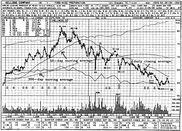
Rather amazingly, these ideas extend to the domain of numerical filters, the topic of this chapter. Numerical filters are just schemes for weighting and summing strings of numbers. Stock prices are typically averaged with numerical filters. The curves in Figure 2 illustrate the daily closing average for Kellogg's common stock and two moving averages. The 50-day moving average is obtained by passing the daily closing average through a numerical filter that averages the most current 50 days' worth of closing averages. The 200-day moving average for the stock price is obtained by passing the daily closing prices through a numerical filter that averages the most current 200 days' worth of daily closing averages. The daily closing averages show fine-grained variation but tend to conceal trends. The 50-day and 200-day averages show less fine-grained variation but give a clearer picture of trends. In fact, this is one of the key ideas in numerical filtering: by selecting our method of averaging, we can filter out fine-grained variations and pass long-term trends (or vice versa), or we can filter out periodic variations and pass nonperiodic variations (or vice versa). Figure 2 illustrates that moving averages typically lag increasing sequences of numbers and lead decreasing sequences. Can you explain why?
We will call any algorithm or procedure for transforming one set of numbers into another set of numbers a numerical filter or digital filter. Digital filters, consisting of memories and arithmetic logic units (ALUs), are implemented in VLSI circuits and used for communication, control, and instrumentation. They are also implemented in random–or semicustom–logic circuits and in programmable microcomputer systems. The inputs to a digital filter are typically electronic measurements that are produced by A/D (analog-to-digital) conversion of the output of an electrical or mechanical sensor. The outputs of the filter are “processed,” “filtered,” or “smoothed” versions of the measurements. In your more advanced courses in electrical and computer engineering you will study signal processing and system theory, assembly language programming, microprocessor system development, and computer design. In these courses you will study the design and programming of hardware that may be used for digital filtering.


