7.3: From Symbols to Binary Codes

Perhaps the most fundamental idea in communication theory is that arbitrary symbols may be represented by strings of binary digits. These strings are called binary words, binary addresses, or binary codes. In the simplest of cases, a finite alphabet consisting of the letters or symbols \(s_{0}, s_{1}, \ldots, s_{M-1}\) is represented by binary codes. The obvious way to implement the representation is to let the \(i^{\text {th }}\) binary code be the binary representation for the subscript \(i\):

\[\begin{gathered}
s_{0} \sim 000=a_{0} \\
s_{1} \sim 001=a_{1} \\
\vdots \\
s_{6} \sim 110=a_{6} \\
s_{7} \sim 111=a_{7} .
\end{gathered} \nonumber \]

The number of bits required for the binary code is \(N\) where

\[2^{N-1}<M \leq 2^{N} \nonumber \]

We say, roughly, that \(N=\log _{2} M\).

Octal Codes

When the number of symbols is large and the corresponding binary codes contain many bits, then we typically group the bits into groups of three and replace the binary code by its corresponding octal code. For example, a seven-bit binary code maps into a three-digit octal code as follows:

\[\begin{gathered}
0000000 \sim 000 \\
0000001 \sim 001 \\
\vdots \\
0100110 \sim 046 \\
\vdots \\
101111 \sim 137 \\
\vdots \\
1111111 \sim 177 .
\end{gathered} \nonumber \]

The octal ASCII codes for representing letters, numbers, and special characters are tabulated in Table 1.

Exercise \(\PageIndex{1}\)

Write out the seven-bit ASCII codes for \(A,q,7\),and {.

Table 1: Octal ASCII Codes (from Donald E. Knuth, The TEXbook, ©1986 by the American Mathematical Society, Providence, Rhode Island p. 367, published by Addison-Wesley Publishing Co.)

	'0	'1	'2	'3	'4	'5	'6	'7
'00x	␀	␁	␂	␃	␄	␅	␆	␇
'01x	␈	␉	␊	␋	␌	␍	␎	␏
'02x	␐	␑	␒	␓	␔	␕	␖	␗
'03x	␘	␙	␚	␛	␜	␝	␞	␟
'04x	␠	!	"	#	$	%	&	'
'05x	(	)	*	+	,	-	.	/
'06x	0	1	2	3	4	5	6	7
'07x	8	9	:	;	<	=	>	?
'10x	@	A	B	C	D	E	F	G
'11x	H	I	J	K	L	M	N	O
'12x	P	Q	R	S	T	U	V	W
'13x	X	Y	Z	[	\	]	^	_
'14x	`	a	b	c	d	e	f	g
'15x	h	i	j	k	l	m	n	o
'16x	p	q	r	s	t	u	v	w
'17x	x	y	z	{	|	}	~	␡

Exercise \(\PageIndex{2}\)

Add a 1 or a 0 to the most significant (left-most) position of the seven-bit ASCII code to produce an eight-bit code that has even parity (even number of 1's). Give the resulting eight-bit ASCII codes and the corresponding three-digit octal codes for %, u, f, 8, and +.

Quantizers and A/D Converters

What if the source alphabet is infinite? Our only hope is to approximate it with a finite collection of finite binary words. For example, suppose the output of the source is an analog voltage that lies between \(−V_0\) and \(+V_0\). We might break this peak-to-peak range up into little voltage cells of size \(\frac{2V}{M} A\) and approximate the voltage in each cell by its midpoint. This scheme is illustrated in Figure 1. In the figure, the cell \(C_i\) is defined to be the set of voltages that fall between \(i_{M^{-} \overline{M}}^{\underline{2} V p V_{\Delta}}\) and \(i^{\underline{2} V} M \Delta+\stackrel{V}{-} M^{\mathrm{A}}\):

\[C_{i}=\left\{V: i . \frac{2 V_{0}}{M}-\frac{V_{0}}{M}<V \leq i \frac{2 V_{0}}{M}+\frac{V_{0}}{M}\right\} \nonumber \]

The mapping from continuous values of \(V\) to a finite set of approximations is

\[Q(V)=i \frac{2 V_{0}}{M}, \text { if } V \in C_{i} \nonumber \]

That is, \(V\) is replaced by the quantized approximation \(i_{M}^{\underline{2} V_{0}}\) whenever \(V\) lies in cell \(C_i\). We may represent the quantized values \(i_{M}^{\underline{2} V_{0}}\) with binary codes by simply representing the subscript of the cell by a binary word. In a subsequent course on digital electronics and microprocessors you will study A/D (analog-to-digital) converters for quantizing variables.

Figure \(\PageIndex{1}\): A Quantizer

Example \(\PageIndex{1}\)

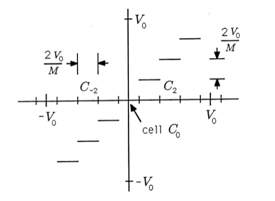
If \(M=8\), corresponding to a three-bit quantizer, we may associate quantizer cells and quantized levels with binary codes as follows:

\(\begin{array}{ll}
V \in C_{-3} & \Rightarrow V_{-3}=(-3) \frac{2 V_{0}}{8} \sim 111 \\
V \in C_{-2} & \Rightarrow V_{-2}=(-2) \frac{2 V_{0}}{8} \sim 110 \\
V \in C_{-1} & \Rightarrow V_{-1}=(-1) \frac{2 V_{0}}{8} \sim 101 \\
V \in C_{0} & \Rightarrow \quad V_{0}=0 \sim 000 \\
V \in C_{1} & \Rightarrow V_{1}=(1) \frac{2 V_{0}}{8} \sim 001 \\
V \in C_{2} & \Rightarrow V_{2}=(2) \frac{2 V_{0}}{8} \sim 010 \\
V \in C_{3} & \Rightarrow V_{3}=(3) \frac{2 V_{0}}{8} \sim 011 .
\end{array}\)

This particular code is called a sign-magnitude code, wherein the most significant bit is a sign bit and the remaining bits are magnitude bits (e.g., \(110 \sim−2\) and \(010 \sim 2\)). One of the defects of the sign-magnitude code is that it wastes one code by using 000 for 0 and 100 for -O. An alternative code that has many other advantages is the 2's complement code. The 2′scomplement codes for positive numbers are the same as the sign-magnitude codes, but the codes for negative numbers are generated by complementing all bits for the corresponding positive number and adding 1:

\(\begin{aligned}
-4 & \sim 100 & \\
-3 &\sim 101 &(100+1) \\
-2 & \sim 110 &(101+1) \\
-1 &\sim 111 &(110+1) \\
0 & \sim 000 \\
1 & \sim 001 \\
2 & \sim 010 \\
3 & \sim 011 .
\end{aligned}\)

Exercise \(\PageIndex{3}\)

Generate the four-bit sign-magnitude and four-bit 2's complement binary codes for the numbers \(-8,-7, \ldots,-1,0,1,2, \ldots, 7\).

Exercise \(\PageIndex{4}\)

Prove that, in the 2's complement representation, the binary codes for \(−n\) and \(+n\) sum to zero. For example,

\[\begin{gathered}
101+011=000 \\
(-3)(3)(0) .
\end{gathered} \nonumber \]

In your courses on computer arithmetic you will learn how to do arithmetic in various binary-coded systems. The following problem illustrates how easy arithmetic is in 2's complement.

Exercise \(\PageIndex{5}\)

Generate a table of sums for all 2's complement numbers between −4 and +3. Show that the sums are correct. Use 0 + 0 = 0, 0 + 1 = 1, 1 + 0 = 1, and 1 + 1 = 0 with a carry into the next bit. For example, 001+001=010.

Binary Trees and Variable-Length Codes

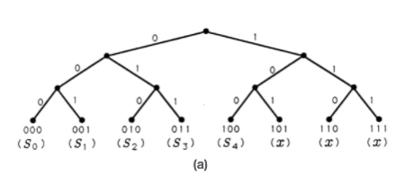
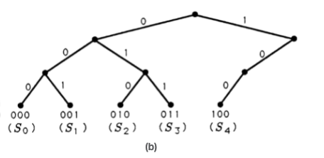
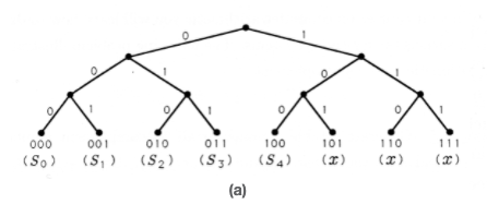
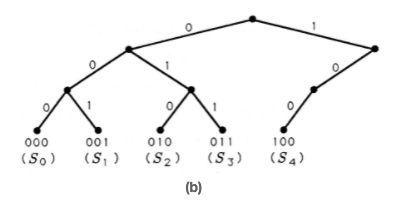
The codes we have constructed so far are constant-length codes for finite alphabets that contain exactly \(M=2^N\) symbols. In the case where \(M=8\) and \(N=3\), then the eight possible three-bit codes may be represented as leaves on the branching tree illustrated in Figure 2(a). The tree grows a left branch for a 0 and a right branch for a 1, until it terminates after three branchings. The three-bit codes we have studied so far reside at the terminating leaves of the binary tree. But what if our source alphabet contains just five symbols or letters? We can represent these five symbols as the three-bit symbols 000 through 100 on the binary tree. This generates a constant-length code with three unused, or illegal, symbols 101 through 111. These are marked with an "\(x\)" in Figure 2(a). These unused leaves and the branches leading to them may be pruned to produce the binary tree of Figure 2(b).

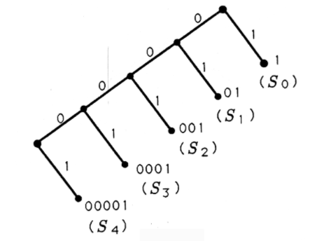
If we admit variable-length codes, then we have several other options for using a binary tree to construct binary codes. Two of these codes and their corresponding binary trees are illustrated in Figure 3. If we disabuse ourselves of the notion that each code word must contain three or fewer bits, then we may construct binary trees like those of Figure 4 and generate their corresponding binary codes. In Figure 4(a), we grow a right branch after each left branch and label each leaf with a code word. In Figure 4(b), we prune off the last right branch and associatea code word with the leaf on the last left branch.

Figure \(\PageIndex{2}\): Binary Trees and Constant-Length Codes; (a) Binary Tree, and (b) Pruned Binary Tree

All of the codes we have generated so far are organized in Table 2. For each code, the average number of bits/symbol is tabulated. This average ranges from 2.4 to 3.0. If all symbols are equally likely to appear, then the best variable-length code would be code 2.

Figure \(\PageIndex{3}\):Binary Trees and Variable-Length Codes; (a) Binary Tree for Variable-length Code, and (b) Another Binary Tree for Variable-length Code

All of the codes we have constructed have a common characteristic: each code word is a terminating leaf on a binary tree, meaning that no code word lies along a limb of branches to another code word. We say that no code word is a prefix to another code word. This property makes each of the codes instantaneously decodable, meaning that each bit in a string of bits may be processed instantaneously (or independently) without dependence on subsequent bits.

Exercise \(\PageIndex{6}\)

Decode the following sequence of bits using code 2:

0111001111000000101100111.

(a)

(b)

Figure \(\PageIndex{4}\): Left-Handed Binary Trees for Variable-Length Codes; (a) Left-handed Binary Tree, and (b) Pruned Binary Tree

Table 2: Variable Length Codes

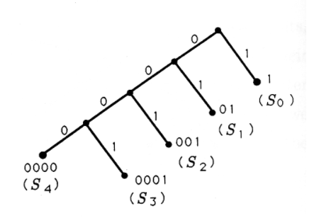
Code #	S0S0	S1S1	S2S2	S3S3	S4S4	Average Bits/Symbol
1	000	001	010	011	100	15/5=3.015/5=3.0
2	000	001	01	10	11	12/5=2.412/5=2.4
3	000	001	010	011	1	13/5=2.613/5=2.6
4	1	01	001	0001	00001	15/5=3.015/5=3.0
5	1	01	001	0001	0000	14/5=2.8

Exercise \(\PageIndex{7}\)

Illustrate the following codes on a binary tree. Which of them are instantaneously decodable? Which can be pruned and remain instantaneously decodable?

\(\begin{array}{ccccc}
S_{0} & S_{1} & S_{2} & S_{3} & S_{4} \\
011 & 100 & 00 & 11 & 101 \\
011 & 100 & 00 & 0 & 01 \\
010 & 000 & 100 & 101 & 111 .
\end{array}\)

Code #2 generated in Table 2 seems like a better code than code #5 because its average number of bits/symbol (2.4) is smaller. But what if symbol \(S_0\) is a very likely symbol and symbol \(S_4\) is a very unlikely one? Then it may well turn out that the average number of bits used by code #5 is less than the average number used by code #2. So what is the best code? The answer depends on the relative frequency of use for each symbol. We explore this question in the next section.