2.7: Signals and Systems Problems

Learning Objectives

• Signals and Systems practice problems.

Complex Number Arithmetic

Find the real part, imaginary part, the magnitude and angle of the complex numbers given by the following expressions.

1. -1
2. \[\frac{1+\sqrt{3}i}{2} \nonumber \]
3. \[1+i+e^{i\tfrac{\pi }{2}} \nonumber \]
4. \[e^{i\tfrac{\pi }{3}}+e^{i\pi }+e^-({i\tfrac{\pi }{3}}) \nonumber \]

Discovering Roots

Complex numbers expose all the roots of real (and complex) numbers. For example, there should be two square-roots, three cube-roots, etc. of any number. Find the following roots.

1. What are the cube-roots of 27? In other words, what is 27^1/3?
2. What are the fifth roots of 3(3^1/5)?
3. What are the fourth roots of one?

Cool Exponentials

1. \[i^{i} \nonumber \]
2. \[i^{2i} \nonumber \]
3. \[i^{i^{-1}} \nonumber \]

Complex-valued Signals

Complex numbers and phasors play a very important role in electrical engineering. Solving systems for complex exponentials is much easier than for sinusoids, and linear systems analysis is particularly easy.

1. Find the phasor representation for each, and re-express each as the real and imaginary parts of a complex exponential. What is the frequency (in Hz) of each? In general, are your answers unique? If so, prove it; if not, find an alternative answer for the complex exponential representation.
   1. \[3\sin (24t) \nonumber \]
   2. \[\sqrt{2} \cos \left ( 2\pi 60t + \frac{\pi }{4} \right ) \nonumber \]
   3. \[2 \cos \left (t + \frac{\pi }{6} \right ) + 4 \sin \left ( t - \frac{\pi }{3} \right ) \nonumber \]
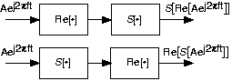
2. Show that for linear systems having real-valued outputs for real inputs, that when the input is the real part of a complex exponential, the output is the real part of the system's output to the complex exponential (see figure below).

\[S\left ( \Re (Ae^{i2\pi ft}) \right ) = \Re \left (S (Ae^{i2\pi ft}) \right ) \nonumber \]

Figure 2.7.1 Complex system

3. For each of the indicated voltages, write it as the real part of a complex exponential \[v(t) = \Re (Ve^{st}) \nonumber \] Explicitly indicate the value of the complex amplitude V and the complex frequency s. Represent each complex amplitude as a vector in the V-plane, and indicate the location of the frequencies in the complex s-plane.
   1. \[v(t) = \cos (5t) \nonumber \]
   2. \[v(t) = \sin \left ( 8t+\frac{\pi }{4} \right ) \nonumber \]
   3. \[v(t) = e^{-t} \nonumber \]
   4. \[v(t) = e^{-(3t)}\sin \left ( 4t+\frac{3\pi }{4} \right ) \nonumber \]
   5. \[v(t) = 5e^{(2t)}\sin (8t + 2\pi ) \nonumber \]
   6. \[v(t) = -2 \nonumber \]
   7. \[v(t) = 4\sin (2t) + 3\cos (2t) \nonumber \]
   8. \[v(t) = 2\cos \left ( 100\pi t + \frac{\pi }{6} \right )- \sqrt{3}\sin \left ( 100\pi t + \frac{\pi }{2} \right ) \nonumber \]
4. Express each of the following signals as a linear combination of delayed and weighted step functions and ramps (the integral of a step).
   1. 
   2. 
   3. 
   4. 
   5. 

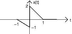
Linear, Time-Invariant Systems

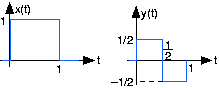
When the input to a linear, time-invariant system is the signal x(t), the output is the signal y(t),

Figure 2.7.2 Time -invariant system

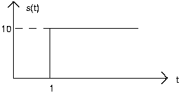
1. Find and sketch this system's output when the input is the depicted signal:
2. Find and sketch this system's output when the input is a unit step.

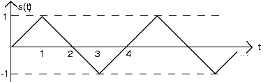
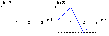
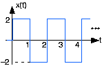
Linear Systems

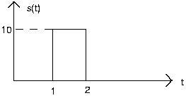
The depicted input x(t) to a linear, time-invariant system yields the output y(t).

Figure 2.7.3 Linear system

1. What is the system's output to a unit step input u(t)?
2. What will the output be when the input is the depicted sqaure wave:

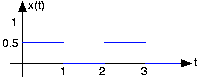
Communication Channel

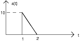
A particularly interesting communication channel can be modeled as a linear, time-invariant system. When the transmitted signal x(t) is a pulse, the received signal r(t) is as shown:

Figure 2.7.4 Communication channel and pulse sequence

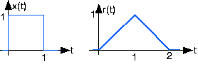
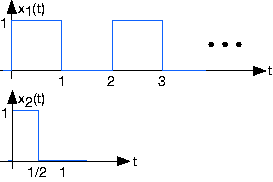
1. What will be the received signal when the transmitter sends the pulse sequence x₁(t)?
2. What will be the received signal when the transmitter sends the pulse sequence x₂(t) that has half the duration as the original?

Analog Computers

So-called analog computers use circuits to solve mathematical problems, particularly when they involve differential equations. Suppose we are given the following differential equation to solve.

\[\frac{\mathrm{d\: y(t)} }{\mathrm{d} t} + ay(t) = x(t) \nonumber \]

In this equation, a is a constant.

1. When the input is a unit step \[(x(t) = u(t)) \nonumber \] the output is given by \[y(t) = (1-e^{-(at)})u(t) \nonumber \] What is the total energy expended by the input?
2. Instead of a unit step, suppose the input is a unit pulse (unit-amplitude, unit-duration) delivered to the circuit at time t =10, what is the output voltage in this case? Sketch the waveform.