5.4: Amplitude Quantization
- Page ID
- 1623
\( \newcommand{\vecs}[1]{\overset { \scriptstyle \rightharpoonup} {\mathbf{#1}} } \)
\( \newcommand{\vecd}[1]{\overset{-\!-\!\rightharpoonup}{\vphantom{a}\smash {#1}}} \)
\( \newcommand{\id}{\mathrm{id}}\) \( \newcommand{\Span}{\mathrm{span}}\)
( \newcommand{\kernel}{\mathrm{null}\,}\) \( \newcommand{\range}{\mathrm{range}\,}\)
\( \newcommand{\RealPart}{\mathrm{Re}}\) \( \newcommand{\ImaginaryPart}{\mathrm{Im}}\)
\( \newcommand{\Argument}{\mathrm{Arg}}\) \( \newcommand{\norm}[1]{\| #1 \|}\)
\( \newcommand{\inner}[2]{\langle #1, #2 \rangle}\)
\( \newcommand{\Span}{\mathrm{span}}\)
\( \newcommand{\id}{\mathrm{id}}\)
\( \newcommand{\Span}{\mathrm{span}}\)
\( \newcommand{\kernel}{\mathrm{null}\,}\)
\( \newcommand{\range}{\mathrm{range}\,}\)
\( \newcommand{\RealPart}{\mathrm{Re}}\)
\( \newcommand{\ImaginaryPart}{\mathrm{Im}}\)
\( \newcommand{\Argument}{\mathrm{Arg}}\)
\( \newcommand{\norm}[1]{\| #1 \|}\)
\( \newcommand{\inner}[2]{\langle #1, #2 \rangle}\)
\( \newcommand{\Span}{\mathrm{span}}\) \( \newcommand{\AA}{\unicode[.8,0]{x212B}}\)
\( \newcommand{\vectorA}[1]{\vec{#1}} % arrow\)
\( \newcommand{\vectorAt}[1]{\vec{\text{#1}}} % arrow\)
\( \newcommand{\vectorB}[1]{\overset { \scriptstyle \rightharpoonup} {\mathbf{#1}} } \)
\( \newcommand{\vectorC}[1]{\textbf{#1}} \)
\( \newcommand{\vectorD}[1]{\overrightarrow{#1}} \)
\( \newcommand{\vectorDt}[1]{\overrightarrow{\text{#1}}} \)
\( \newcommand{\vectE}[1]{\overset{-\!-\!\rightharpoonup}{\vphantom{a}\smash{\mathbf {#1}}}} \)
\( \newcommand{\vecs}[1]{\overset { \scriptstyle \rightharpoonup} {\mathbf{#1}} } \)
\( \newcommand{\vecd}[1]{\overset{-\!-\!\rightharpoonup}{\vphantom{a}\smash {#1}}} \)
- Analog-to-digital conversion.
The Sampling Theorem says that if we sample a bandlimited signal s(t) fast enough, it can be recovered without error from its samples
\[s(nT_{s}),n\in \left \{ ...,-1,0,1,... \right \} \nonumber \]
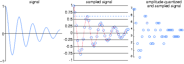
Sampling is only the first phase of acquiring data into a computer: Computational processing further requires that the samples be quantized: analog values are converted into digital form. In short, we will have performed analog-to-digital (A/D) conversion.


A phenomenon reminiscent of the errors incurred in representing numbers on a computer prevents signal amplitudes from being converted with no error into a binary number representation. In analog-to-digital conversion, the signal is assumed to lie within a predefined range. Assuming we can scale the signal without affecting the information it expresses, we'll define this range to be [-1,1]. Furthermore, the A/D converter assigns amplitude values in this range to a set of integers. A B-bit converter produces one of the integers
\[\left \{0,1,...,2^{B} -1\right \} \nonumber \]
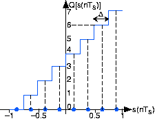
for each sampled input. Figure 5.4.1 shows how a three-bit A/D converter assigns input values to the integers. We define a quantization interval to be the range of values assigned to the same integer. Thus, for our example three-bit A/D converter, the quantization interval Δ is 0.25; in general, it is 2/2B.
Recalling the plot of average daily highs in this frequency domain problem, why is this plot so jagged? Interpret this effect in terms of analog-to-digital conversion.
Solution
The plotted temperatures were quantized to the nearest degree. Thus, the high temperature's amplitude was quantized as a form of A/D conversion.
Because values lying anywhere within a quantization interval are assigned the same value for computer processing, the original amplitude value cannot be recovered without error. Typically, the D/A converter, the device that converts integers to amplitudes, assigns an amplitude equal to the value lying halfway in the quantization interval. The integer 6 would be assigned to the amplitude 0.625 in this scheme. The error introduced by converting a signal from analog to digital form by sampling and amplitude quantization then back again would be half the quantization interval for each amplitude value. Thus, the so-called A/D error equals half the width of a quantization interval: 1/2B. As we have fixed the input-amplitude range, the more bits available in the A/D converter, the smaller the quantization error.
To analyze the amplitude quantization error more deeply, we need to compute the signal-to-noise ratio, which equals the ratio of the signal power and the quantization error power. Assuming the signal is a sinusoid, the signal power is the square of the rms amplitude:
\[power(s)=\left ( \frac{1}{\sqrt{2}} \right )^{2}=\frac{1}{2} \nonumber \]
The Figure 5.4.2 details a single quantization interval.

Its width is \(Δ\) and the quantization error is denoted by \(\varepsilon\). To find the power in the quantization error, we note that no matter into which quantization interval the signal's value falls, the error will have the same characteristics. To calculate the rms value, we must square the error and average it over the interval.
\[\begin{align*} rms(\varepsilon) &=\sqrt{\frac{1}{\Delta }\int_{-\Delta }^{\Delta }\varepsilon ^{2}d\varepsilon } \\[4pt] &=\left ( \frac{\Delta ^{2}}{12} \right )^{\frac{1}{2}} \end{align*} \]
Since the quantization interval width for a B-bit converter equals
\[\dfrac{2}{2^{B}}=2^{-(B-1)} \nonumber \]
we find that the signal-to-noise ratio for the analog-to-digital conversion process equals
\[SNR=\frac{\frac{1}{2}}{\frac{2^{-(2(B-1))}}{12}}=\frac{3}{2}2^{2B}=6B+\log 1.5dB \nonumber \]
Thus, every bit increase in the A/D converter yields a 6 dB increase in the signal-to-noise ratio. The constant term 10 log1.5 equals 1.76.
This derivation assumed the signal's amplitude lay in the range [-1,1]. What would the amplitude quantization signal-to-noise ratio be if it lay in the range [-A,A]?
Solution
The signal-to-noise ratio does not depend on the signal amplitude. With an A/D range of [-A,A] the quantization interval
\[\Delta =\frac{2A}{2^{B}} \nonumber \]
and the signal's rms value (again assuming it is a sinusoid) is
\[\frac{A}{\sqrt{2}} \nonumber \]
How many bits would be required in the A/D converter to ensure that the maximum amplitude quantization error was less than 60 db smaller than the signal's peak value?
Solution
Solving
\[2^{-B}=0.001 \nonumber \]
results in
\[B=10\; bits \nonumber \]
Music on a CD is stored to 16-bit accuracy. To what signal-to-noise ratio does this correspond?
Solution
A 16-bit A/D converter yields a SNR of
\[6\times 16+10\log 1.5=97.8dB \nonumber \]
Once we have acquired signals with an A/D converter, we can process them using digital hardware or software. It can be shown that if the computer processing is linear, the result of sampling, computer processing, and unsampling is equivalent to some analog linear system. Why go to all the bother if the same function can be accomplished using analog techniques? Knowing when digital processing excels and when it does not is an important issue.


