1.9: The Mass-Damper-Spring System - A 2nd Order LTI System and ODE

Last updated
Save as PDF

Page ID: 21147

\( \newcommand{\vecs}[1]{\overset { \scriptstyle \rightharpoonup} {\mathbf{#1}} } \) \( \newcommand{\vecd}[1]{\overset{-\!-\!\rightharpoonup}{\vphantom{a}\smash {#1}}} \)\(\newcommand{\id}{\mathrm{id}}\) \( \newcommand{\Span}{\mathrm{span}}\) \( \newcommand{\kernel}{\mathrm{null}\,}\) \( \newcommand{\range}{\mathrm{range}\,}\) \( \newcommand{\RealPart}{\mathrm{Re}}\) \( \newcommand{\ImaginaryPart}{\mathrm{Im}}\) \( \newcommand{\Argument}{\mathrm{Arg}}\) \( \newcommand{\norm}[1]{\| #1 \|}\) \( \newcommand{\inner}[2]{\langle #1, #2 \rangle}\) \( \newcommand{\Span}{\mathrm{span}}\) \(\newcommand{\id}{\mathrm{id}}\) \( \newcommand{\Span}{\mathrm{span}}\) \( \newcommand{\kernel}{\mathrm{null}\,}\) \( \newcommand{\range}{\mathrm{range}\,}\) \( \newcommand{\RealPart}{\mathrm{Re}}\) \( \newcommand{\ImaginaryPart}{\mathrm{Im}}\) \( \newcommand{\Argument}{\mathrm{Arg}}\) \( \newcommand{\norm}[1]{\| #1 \|}\) \( \newcommand{\inner}[2]{\langle #1, #2 \rangle}\) \( \newcommand{\Span}{\mathrm{span}}\)\(\newcommand{\AA}{\unicode[.8,0]{x212B}}\)

Consider a rigid body of mass \(m\) that is constrained to sliding translation \(x(t)\) in only one direction, Figure \(\PageIndex{1}\). The mass is subjected to an externally applied, arbitrary force \(f_x(t)\), and it slides on a thin, viscous, liquid layer that has linear viscous damping constant \(c\). Additionally, the mass is restrained by a linear spring. The force exerted by the spring on the mass is proportional to translation \(x(t)\) relative to the undeformed state of the spring, the constant of proportionality being \(k\). Parameters \(m\), \(c\), and \(k\) are positive physical quantities. All of the horizontal forces acting on the mass are shown on the FBD of Figure \(\PageIndex{1}\).

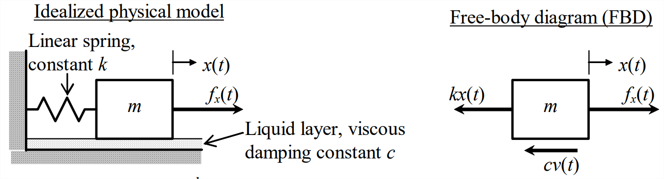
Figure \(\PageIndex{1}\): 2^nd order mass-damper-spring mechanical system.

From the FBD of Figure \(\PageIndex{1}\) and Newton’s 2^nd law for translation in a single direction, we write the equation of motion for the mass:

\[\sum(\text { Forces })_{x}=\text { mass } \times(\text { acceleration })_{x} \nonumber \]

where \((acceleration)_{x}=\dot{v}=\ddot{x};\)

\[f_{x}(t)-c v-k x=m \dot{v}. \nonumber \]

Re-arrange this equation, and add the relationship between \(x(t)\) and \(v(t)\), \(\dot{x}\) = \(v\):

\[m \dot{v}+c v+k x=f_{x}(t)\label{eqn:1.15a} \]

\[\dot{x}-v=0\label{eqn:1.15b} \]

Equations \(\ref{eqn:1.15a}\) and \(\ref{eqn:1.15b}\) are a pair of 1^st order ODEs in the dependent variables \(v(t)\) and \(x(t)\). The two ODEs are said to be coupled, because each equation contains both dependent variables and neither equation can be solved independently of the other. Such a pair of coupled 1st order ODEs is called a 2nd order set of ODEs.

Solving 1st order ODE Equation 1.3.3 in the single dependent variable \(v(t)\) for all times \(t\) > \(t_0\) requires knowledge of a single IC, which we previously expressed as \(v_0 = v(t_0)\). Similarly, solving the coupled pair of 1^st order ODEs, Equations \(\ref{eqn:1.15a}\) and \(\ref{eqn:1.15b}\), in dependent variables \(v(t)\) and \(x(t)\) for all times \(t\) > \(t_0\), requires a known IC for each of the dependent variables:

\[v_{0} \equiv v\left(t_{0}\right)=\dot{x}\left(t_{0}\right) \text { and } x_{0}=x\left(t_{0}\right)\label{eqn:1.16} \]

In this book, the mathematical problem is expressed in a form different from Equations \(\ref{eqn:1.15a}\) and \(\ref{eqn:1.15b}\): we eliminate \(v\) from Equation \(\ref{eqn:1.15a}\) by substituting for it from Equation \(\ref{eqn:1.15b}\) with \(v = \dot{x}\) and the associated derivative \(\dot{v} = \ddot{x}\), which gives¹

\[m \ddot{x}+c \dot{x}+k x=f_{x}(t)\label{eqn:1.17} \]

ODE Equation \(\ref{eqn:1.17}\) is clearly linear in the single dependent variable, position \(x(t)\), and time-invariant, assuming that \(m\), \(c\), and \(k\) are constants. The highest derivative of \(x(t)\) in the ODE is the second derivative, so this is a 2^nd order ODE, and the mass-damper-spring mechanical system is called a 2^nd order system. If \(f_x(t)\) is defined explicitly, and if we also know ICs Equation \(\ref{eqn:1.16}\) for both the velocity \(\dot{x}(t_0)\) and the position \(x(t_0)\), then we can, at least in principle, solve ODE Equation \(\ref{eqn:1.17}\) for position \(x(t)\) at all times \(t\) > \(t_0\). We shall study the response of 2^nd order systems in considerable detail, beginning in Chapter 7, for which the following section is a preview.

¹An alternative derivation of ODE Equation \(\ref{eqn:1.17}\) is presented in Appendix B, Section 19.2. The rate of change of system energy is equated with the power supplied to the system.