4.3: Frequency Response of the First Order Damper-Spring System

To extract the steady-state sinusoidal response \(x_{ss}(t)\) from total response Equation 4.2.7, we drop the transient, exponential decay terms:

\[x_{s s}(t)=\frac{F}{k}\left(\frac{1}{1+\left(\omega \tau_{1}\right)^{2}}\right)\left(\cos \omega t+\omega \tau_{1} \sin \omega t\right)\label{eqn:4.5} \]

We can write Equation \(\ref{eqn:4.5}\) in a form that is more physically expressive by using some algebraic manipulation and the general trigonometric identity,

\[\cos \theta \times \cos \phi-\sin \theta \times \sin \phi=\cos (\theta+\phi)\label{eqn:4.6} \]

The algebraic manipulation involves the sinusoidally varying terms of Equation \(\ref{eqn:4.5}\). For generality, let us assume that each term is multiplied by a general coefficient, \(C\) or \(-S\), so that those terms can be written and manipulated as

\[C \cos \omega t-S \sin \omega t=\sqrt{C^{2}+S^{2}}\left(\cos \omega t \frac{C}{\sqrt{C^{2}+S^{2}}}-\sin \omega t \frac{S}{\sqrt{C^{2}+S^{2}}}\right) \nonumber \]

Now we identify the coefficients of \(\cos \omega t\) and \(\sin \omega t\) inside parentheses as themselves representing trigonometric functions: \(\frac{C}{\sqrt{C^{2}+S^{2}}} \equiv \cos \phi\) and \(\frac{S}{\sqrt{C^{2}+S^{2}}} \equiv \sin \phi\), where angle \(\phi\) is given by a four-quadrant tangent function,

\[\phi=\tan ^{-1}\left(\frac{S}{C}\right)\label{eqn:4.7} \]

Figure \(\PageIndex{1}\)

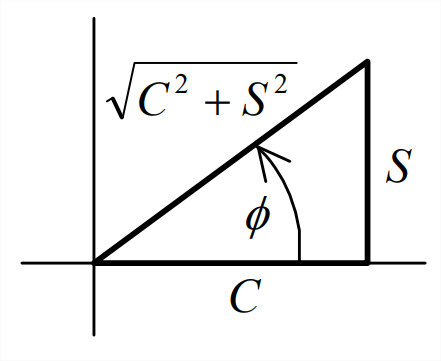
These trigonometric relations are illustrated at left on the drawing of a right triangle.

So, with identity Equation \(\ref{eqn:4.6}\), the trigonometric sum becomes

\[C \cos \omega t-S \sin \omega t=\sqrt{C^{2}+S^{2}}(\cos \omega t \cos \phi-\sin \omega t \sin \phi)=\sqrt{C^{2}+S^{2}} \cos (\omega t+\phi)\label{eqn:4.8} \]

Associating Equation \(\ref{eqn:4.5}\) with Equation \(\ref{eqn:4.8}\), we have \(C=1\), \(S=-\omega \tau_{1}\). Therefore, Equation \(\ref{eqn:4.5}\) becomes

\[x_{s s}(t)=\frac{F}{k}\left(\frac{1}{1+\left(\omega \tau_{1}\right)^{2}}\right) \sqrt{1+\left(\omega \tau_{1}\right)^{2}} \cos (\omega t+\phi) \nonumber \]

\[x_{s s}(t)=\frac{F}{k} \frac{1}{\sqrt{1+\left(\omega \tau_{1}\right)^{2}}} \cos (\omega t+\phi) \equiv X(\omega) \cos (\omega t+\phi(\omega)), \quad \phi(\omega)=\tan ^{-1}\left(\frac{-\omega \tau_{1}}{1}\right)\label{eqn:4.9} \]

Let us compare the steady-state response (output), \(x_{s s}(t)\) of Equation \(\ref{eqn:4.9}\), with the excitation (input), \(f_{x}(t)=F \cos \omega t\). The magnitude of response, which is a function of excitation frequency \(\omega\), is

\[X(\omega)=\frac{F}{k} \frac{1}{\sqrt{1+\left(\omega \tau_{1}\right)^{2}}}\label{eqn:4.10} \]

We will often deal with the magnitude ratio, defined as the magnitude of response divided by the magnitude of excitation,

\[\frac{X(\omega)}{F}=\frac{1}{k} \frac{1}{\sqrt{1+\left(\omega \tau_{1}\right)^{2}}}\label{eqn:4.11} \]

The phase (or phase angle, since it is an angle in radians or degrees) of response relative to the phase of the excitation is also a function of excitation frequency \(\omega\):

\[\phi(\omega)=\tan ^{-1}\left(-\omega \tau_{1}\right)\label{eqn:4.12} \]

In general, if phase angle \(\phi\) is positive, 0° < \(\phi\) < 180°, it is called a phase lead, because the peaks and zeros of the response occur in time before those of the excitation. If phase angle \(\phi\) is negative, −180° ≤ \(\phi\) < 0°, it is called a phase lag, because the peaks and zeros of the response occur in time after those of the excitation. The response is said to be in-phase if \(\phi\) = 0° exactly, and out-of-phase if \(\phi\) = −180° exactly. For the standard stable 1^st order system considered presently, \(\phi(\omega)=\tan ^{-1}\left(-\omega \tau_{1}\right)\), which is a phase lag, always negative in the 4^th quadrant, −90° < \(\phi\) < 0°, with \(\phi\rightarrow\) 0° for very small \(\omega\) and \(\phi\rightarrow\)-90° for very large \(\omega\).

The frequency-response function (abbreviated FRF) is considered to consist of both the magnitude ratio, Equation \(\ref{eqn:4.11}\) in this case, and the phase angle, Equation \(\ref{eqn:4.12}\) in this case. We will see later that both of these functions can be expressed together in a mathematical equation as a single complex function of frequency. It is common in engineering practice to plot these two real functions of frequency \(\omega\) on a pair of over-and-under graphs in the format of Figure \(\PageIndex{2}\), which represents Equations \(\ref{eqn:4.11}\) and \(\ref{eqn:4.12}\) specifically. This format is a type of Bode diagram (after Hendrik Wade Bode, American mathematician, physicist, and control-system engineer, 1905-1982).

Figure \(\PageIndex{2}\): Frequency-response function of 1^st order damper-spring system

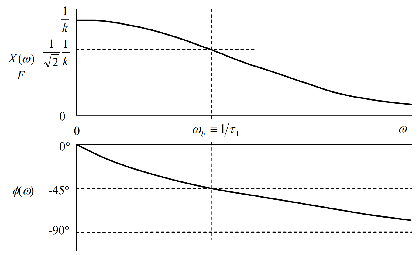
The break frequency \(\omega_{b} \equiv 1 / \tau_{1}\) is shown explicitly on Figure \(\PageIndex{2}\). There is no obvious “break” in the curves of Figure \(\PageIndex{2}\); but a break does indeed exist, the form of which will be revealed in the following discussion.

To represent frequency response over broad bands of frequency, the magnitude ratio and phase are often plotted versus the logarithm of frequency. Moreover, to allow the possibility of very large dynamic ranges of magnitude response, the magnitude ratio itself is often plotted on a logarithmic scale, making the magnitude ratio a log-log graph, where “log” denotes logarithm to the base 10. On such a graph, it is often possible to construct straight-line asymptotes that are useful for describing the variation with frequency of the magnitude. To illustrate this for the 1^st order system, we re-write Equation \(\ref{eqn:4.11}\) as a dimensionless ratio and, for clarity of expression, use the definition \(\omega_{b} \equiv 1 / \tau_{1}\), and then take the logarithm:

\[\frac{X(\omega)}{F / k}=\frac{1}{\sqrt{1+\left(\omega \tau_{1}\right)^{2}}}=\frac{1}{\sqrt{1+\left(\omega / \omega_{b}\right)^{2}}}=\frac{1}{\sqrt{1+\left(f / f_{b}\right)^{2}}}\label{eqn:4.13a} \]

\[\log \left(\frac{X(\omega)}{F / k}\right)=\log \left(\frac{1}{\sqrt{1+\left(\omega / \omega_{b}\right)^{2}}}\right)=-\frac{1}{2} \log \left[1+\left(\frac{\omega}{\omega_{b}}\right)^{2}\right]=-\frac{1}{2} \log \left[1+\left(\frac{f}{f_{b}}\right)^{2}\right]\label{eqn:4.13b} \]

In the last versions on the right-hand sides of Equations \(\ref{eqn:4.13a}\) and \(\ref{eqn:4.13b}\), we have used \(\omega \equiv 2 \pi f\) and \(\omega_{b} \equiv 2 \pi f_{b}\) in order to express the equation in terms of cyclic frequency. The low-frequency asymptote is the limit of Equation \(\ref{eqn:4.13b}\) as the frequency \(\rightarrow\) 0 from above:

\[\lim _{\omega \rightarrow 0}\left[\log \left(\frac{X(\omega)}{F / k}\right)\right]=-\frac{1}{2} \log (1)=0\label{eqn:4.14} \]

The high-frequency asymptote is the limit of Equation \(\ref{eqn:4.13b}\) as the frequency \(\rightarrow\inf\) from below:

\[\lim _{\omega \rightarrow \infty}\left[\log \left(\frac{X(\omega)}{F / k}\right)\right]=-\frac{1}{2} \log \left[\left(\frac{\omega}{\omega_{b}}\right)^{2}\right]=-\log \left(\frac{\omega}{\omega_{b}}\right)=-\log \left(\frac{f}{f_{b}}\right)\label{eqn:4.15} \]

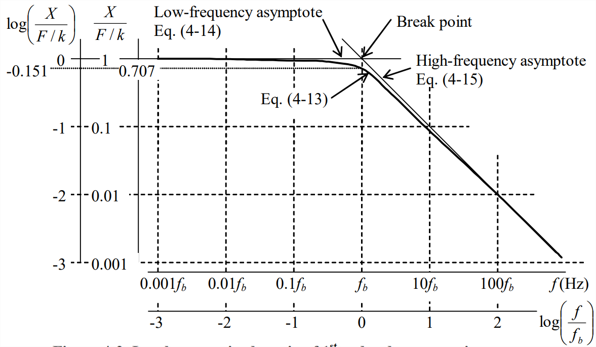
Figure \(\PageIndex{3}\) on the next page is a log-log graph of Equations \(\ref{eqn:4.13a}\) and \(\ref{eqn:4.13b}\) that shows the asymptotes Equation \(\ref{eqn:4.14}\) and Equation \(\ref{eqn:4.15}\). Notice that on the log-log scale, the low-frequency asymptote is a good approximation for the actual function at frequencies \(f<f_{b_{j}}\), and the high-frequency asymptote is a good approximation for the actual function at frequencies \(f>f_{b_{j}}\). The intersection of the two asymptotes is called the break (or corner) because it is a change in slope of the asymptotic approximations to the actual function. The break (or corner) frequency is denoted \(f_b\). For this 1^st order system at \(f_{b}=\omega_{b} / 2 \pi=1 /\left(2 \pi \tau_{1}\right)\), the magnitude of response is reduced to \(1 / \sqrt{2}\) of its static (\(f\) = 0) value, and the phase is -45° (see also Figure \(\PageIndex{2}\)).

The high-frequency asymptote on Figure \(\PageIndex{2}\) merits some additional comment. Note that its slope on the log-log scale equals –1, i.e., the magnitude shrinks one decade (order of magnitude) for each decade increase in the frequency. Frequency response magnitude ratios are often given in decibels (dB), especially in acoustics for sound pressure level. A magnitude ratio in decibels is defined to be 20 × \(\log\)(magnitude ratio). If the magnitude ratio on Figure \(\PageIndex{2}\) had been plotted in decibels versus \(\log\)(frequency), then the slope of the high-frequency asymptote would be –20; this is often referred to as a 20 dB/decade rolloff of the magnitude ratio.

Another observation worth making, especially from Figure \(\PageIndex{2}\), is that the standard 1^st order system considered here behaves like a mild low-pass filter: the system responds most sensitively to excitation at frequencies below the break frequency, the magnitude of response being about equal to the static response. However, at excitation frequencies above the break frequency, the system responds much less sensitively, and the magnitude of response diminishes progressively as the excitation frequency increases.

Figure \(\PageIndex{3}\): Log-log magnitude ratio of 1^st order damper-spring system