7.7: Chapter 7 Homework

1. A particular device is known to be an LTI mass-spring system having negligible damping. It is required that stiffness constant \(k\) and mass \(m\) be identified experimentally. First, a static force of 100 N is applied through a string tied to the mass, producing a static translation of the mass. Next, the string is cut cleanly, allowing the system to vibrate freely from the initial static translation (with zero initial velocity). The subsequent motion is measured by an accelerometer, a sensor that is attached to the system mass and measures, of course, translational acceleration of the mass. The measured acceleration is described with good accuracy by the equation \[a(t) \equiv \ddot{x}(t)=-4.93 \cos (10 \pi t) \frac{\mathrm{m}}{\mathrm{sec}^{2}}, \text { for } 0<t, \text { with } t \text { in seconds } \nonumber \]

   

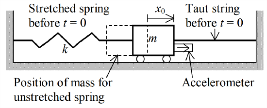
   Figure \(\PageIndex{1}\)

   1. Differentiate twice Equation 7.3.4 for displacement, \(x(t)=x_{\max } \cos \left(\omega_{n} t+\phi\right)\): first, to derive the associated equation for velocity, \(v(t)=\dot{x}(t)\); and second, to derive the associated equation for acceleration, \(a(t)=\dot{v}(t)=\ddot{x}(t)\).
   2. From the experimental data given previously and your results in part 7.1.1, infer values (with units) for stiffness constant \(k\) and mass \(m\).
2. Consider again the reaction wheel assembly introduced in Section 3.3 (Figure 3.3.1), but now suppose that there is a rotational spring with stiffness constant \(k_{\theta}\) connecting the shaft to a rigid wall. Also, for this problem only, assume that the bearing viscous damping torque is negligible.

   

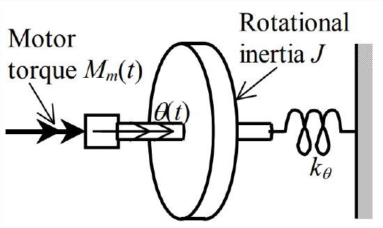
   Figure \(\PageIndex{2}\)

   1. Sketch a rotational FBD (similar to that in Section 3.3, but with appropriate differences), then apply Newton’s 2^nd law for rotation to derive the 2^nd order ODE for wheel rotation \(\theta(t)\). This ODE should have the form of Equation 7.1.2, but with the notation appropriate for this system.
   2. Convert the ODE of part 7.2.1 into the standard form Equation 7.1.5, \(\ddot{\theta}+\omega_{n}^{2} \theta=\omega_{n}^{2} u(t)\). Write specific equations (in terms of this system’s parameters and notation) for natural frequency \(\omega_{n}\) and input quantity \(u(t)\).
   3. The electric torque motor that drives the rotor generates 4.00 oz-inch of torque per amp of electrical current (1 lb = 16 oz). According to the motor manufacturer, the current should be limited to 5.00 A or less in order to avoid toasting the motor, so the maximum motor torque is 20.0 oz-inch. Suppose that this maximum torque is applied to the rotor as a step function. It is required that the subsequent rotation angle \(\theta(t)\) of the rotor not exceed 45°. Calculate the minimum stiffness constant \(k_{\theta}\) (units of lb-inch/rad) that will limit the step response \(\theta(t)\) to 45° or less. Also, calculate the natural frequency in Hz of the system with this value of \(k_{\theta}\). The rotor has rotational inertia \(J\) = 2.56e−3 lb-s²-inch.
3. In the test laboratory of a spacecraft manufacturer, a vibration-isolation platform is supported on a flexible foundation so that the vibration induced by traffic on a busy nearby freeway will not disturb functional testing of delicate space-qualified components. The platform weighs 907 kg_f, and the flexible foundation has nominal stiffness constant \(k\) = 3,440 kN/m.

   

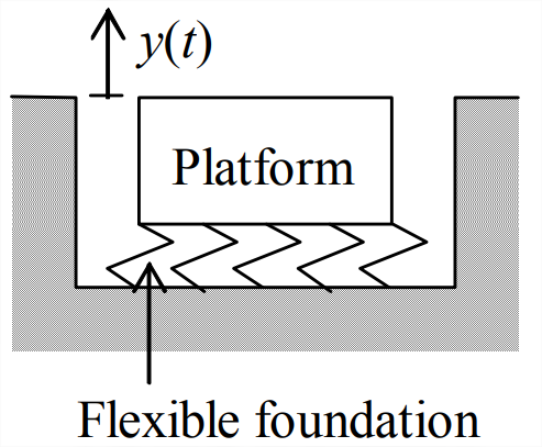
   Figure \(\PageIndex{3}\)

   1. Calculate the predicted values of system natural frequency in rad/s and Hz, and system natural period \(T_{n}\). Recall from Section 3.2 that the kg_f is not a consistent unit in the SI system. (partial answer: \(\omega_{n}\) = 61.6 rad/s)
   2. In a test to determine precisely the dynamic characteristics of this mass-spring system (having negligible damping), the platform is to be given initial downward displacement \(y(0)\) = −0.104 mm (relative to the static equilibrium position) and initial upward velocity \(\dot{y}(0)\) = +7.20 mm/s. The platform will then be allowed to vibrate freely. Write the numerical algebraic equation for the predicted response \(y(t)\) in mm.
4. Consider the rolling motion of a balloon carrying a basket, with the vehicle neither ascending nor descending¹. Weight \(W\) of the vehicle acts downward through the vehicle’s center of gravity \(G\), and buoyancy force \(W\) acts upward through center of buoyancy \(M\), which is the center of gravity of the volume of air displaced by the vehicle. We denote as \(R\) the separation of \(G\) and \(M\) in the vehicle’s plane of symmetry. Note that with \(M\) above \(G\), weight and buoyancy form a stabilizing couple moment, the moment arm being \(R \sin \theta\). Suppose that wind, gusts, and possibly other forms of disturbance and control exert an externally applied rolling moment about \(G\), which is denoted as \(M_{r}(t)\). Denote the vehicle’s rotational inertia about \(G\) as \(J_{G}\). Assume that the vehicle rolls about point \(G\), as if there were a frictionless hinge at \(G\), and neglect all sources of damping.

   

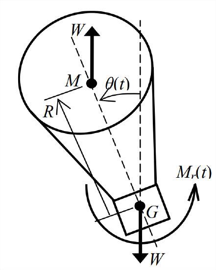
   Figure \(\PageIndex{4}\)

   1. Apply Newton’s 2^nd law for rotation to derive the linearized 2^nd order ODE for roll angle \(\theta(t)\), assumed to be sufficiently small that \(\sin \theta \approx \theta\) radians. This ODE should have the form of Equation 7.1.2, but with the notation appropriate for this system.
   2. Convert the ODE of part 7.4.1 into the standard form Equation 7.1.5, \(\ddot{\theta}+\omega_{n}^{2} \theta=\omega_{n}^{2} u(t)\). Write specific equations (in terms of this system’s parameters and notation) for rolling natural frequency \(\omega_{n}\) and standard input variable \(u(t)\). (partial answer: \(\omega_{n}=\sqrt{W R / J_{G}}\))
5. (Adapted from Craig, 1981, Problem 5.1 on page 120) In single-engine, high-wing, general-aviation airplanes, the structures of the main landing gears are usually simple tilted cantilever beams, as illustrated in the drawing at right. When this type of airplane touches down in a landing, the beams, in combination with the flexible tires, constitute a structural spring that cushions the landing impact.

   

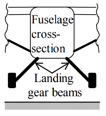
   Figure \(\PageIndex{5}\)

   The drawings below show a simplified model used to study landing impact of a light airplane, with mass \(m\) being that of the airplane body, and stiffness \(k\) being that of the landing gear beams and tires. (The model also represents a person bouncing passively on a pogo stick.) The airplane’s sinking speed just before touchdown is denoted as \(V\), and \(g\) is the acceleration of gravity. Let us call the instant of tire contact \(t = 0\) and measure the airplane’s downward vertical motion \(y(t)\) relative to its position at that instant, as indicated on the right-hand drawing. Hence, the initial conditions are \(y(0)= 0\) and \(\dot{y}(0)=V\).

   

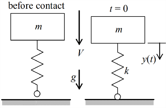
   Figure \(\PageIndex{6}\)

   1. Sketch a FBD of the forces acting upon \(m\) during the time of tire contact with the ground, and use that FBD and Newton’s 2^nd law to write the 2^nd order ODE of motion for \(y(t)\). Note in this case that we measure motion relative to the spring-undeformed position, not relative to the static equilibrium position, so it is necessary to include the body weight \(W = mg\) on the FBD.
   2. Put the ODE of motion into standard form. Now combine both the IC solution (since \(\dot{y}(0)=V>0\)) and the step-response solution (since \(W\) is essentially a step input) that are derived in Section 7.3 to write the algebraic equation for the response \(y(t)\) during the time of tire contact. Express this equation in the form \(y(t)=C_{1}+C_{2} \sin \left(\omega_{n} t-C_{3}\right)\), where the \(C_i\) and \(\omega_{n}\) are positive constants that you should define in terms of the given algebraic parameters. You should find useful the trigonometric identity \(\sin A \cos B \pm \cos A \sin B=\sin (A \pm B)\). If necessary, review the procedure in Section 4.3, Equations 4.3.2, 4.3.4, and 4.3.5, for combining sines and cosines.
   3. Use the correct result from part 7.5.2 above to sketch a time history of the response \(y(t)\) during the time of tire contact. To make it relatively easy to sketch, suppose that the landing is hard, with \(V / \omega_{n}=\sqrt{3} W / k\), and show that \(y(t)=(W / k)\left[1+2 \sin \left(\omega_{n} t-30^{\circ}\right)\right]\). From your \(y(t)\) equation and sketch, infer general algebraic equations (not applicable only for \(V / \omega_{n}=\sqrt{3} W / k\)) for the maximum value \(y_{\max }\), the time at which \(y(t)=y_{\max }\), and the time at which the tires loses contact with the ground upon rebound. For what range of landing impact velocities \(V\) does this theory predict that the tires will lose ground contact upon rebound? Is this theory completely realistic?
6. The ideal LC circuit² drawn below is a series combination of a voltage source \(e_{i}(t)\), an ideal inductor (having only inductance \(L\), no resistance), and a capacitor with capacitance \(C\). Recall that the current is the rate of change of charge \(q(t)\) on the capacitor, \(i=d q / d t\). Apply Kirchhoff’s voltage law, as in Electricity Example 5.2.4 of Section 5.2, and show that the ODE for \(q(t)\) is \(L \ddot{q}+(1 / C) q=e_{i}(t)\). Convert this ODE into the standard 2^nd order form Equation 7.1.5, \(\ddot{q}+\omega_{n}^{2} q=\omega_{n}^{2} u(t)\); write specific equations [in terms of \(L\), \(C\), and \(e_{i}(t)\)] for natural frequency \(\omega_{n}\) and input quantity \(u(t)\).

   

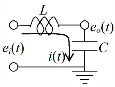
   Figure \(\PageIndex{7}\)

7. The circuit³ drawn at right consists of three stages, each built around an op-amp, and there is feedback of voltage \(e_{f}(t)\) from the last (righthand) stage to the first (lefthand) stage, where the input voltage \(e_{i}(t)\) is applied. The circuit output voltage, \(e_{o}(t)\), is the output of the middle stage. For the first stage, a summing, inverting integrator, use the methods of Chapter 5 to derive the first ODE, \(e_{f} / R_{1 f}+e_{i} / R_{1 i}=-C_{1} \dot{e}_{m}\). Next, for the middle stage, an inverting integrator, derive the second ODE, \(e_{m} / R_{2}=-C_{2} \dot{e}_{o}\) (homework Problem 5.6). Now differentiate the second ODE and use the result to substitute for \(\dot{e}_{m}\) in the first ODE. The last stage is a simple sign inverter, for which \(e_{f}=-e_{o}\) from Equation 5.3.5. Substitute for \(e_{f}\) and show that the ODE relating output voltage \(e_{o}(t)\) to input voltage \(e_{i}(t)\) for the entire circuit is \(\ddot{e}_{o}+\frac{1}{R_{2} C_{2} R_{1 f} C_{1}} e_{o}=\frac{1}{R_{2} C_{2} R_{1 f} C_{1}} \frac{R_{1 f}}{R_{1 i}} e_{i}\). Convert this ODE into the standard 2^nd order form Equation 7.1.5, \(\ddot{e}_{o}+\omega_{n}^{2} e_{o}=\omega_{n}^{2} u(t)\); write specific equations (in terms of this circuit’s resistances, capacitances, and input voltage) for natural frequency \(\omega_{n}\) and input quantity \(u(t)\).

   

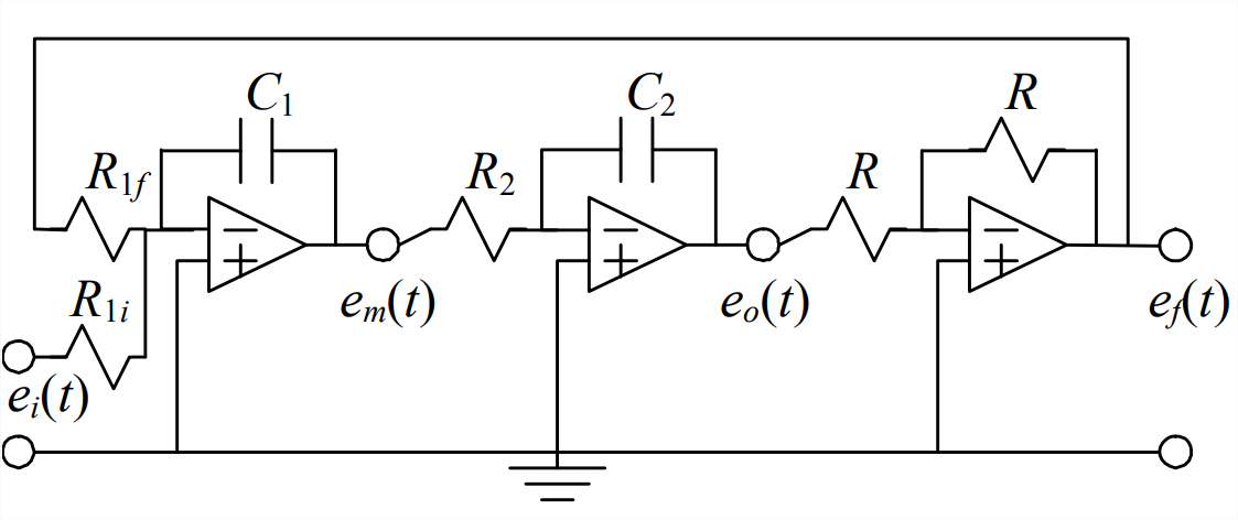
   Figure \(\PageIndex{8}\)

8. If you compare the experimental results for a beam that are presented in Example Problem 7.6.1 with the ideal theoretical results presented in Example Problem 7.6.2, you will observe that there are some significant differences between the two sets of results. In this problem, you will investigate some reasons for those differences.
   1. The beam of Figure 7.6.1 is an extruded aluminum “flat”. Due to manufacturing imperfections, its cross section is not completely uniform (constant) along the length; however, students made the following careful measurements of average cross-sectional dimensions: width \(b\) = 2.00 inches, depth \(h\) = 0.120 inch. The students also measured the average weight per unit length of 0.0230 lb/inch. Using this information, calculate the “actual” average weight density \(w\) in lb/inch³, and compare your value with the standard (in preliminary-design calculations) value for aluminum, 0.1000 lb/inch3 , which is used in Example Problem 7.6.2. Also, calculate the total weight of the beam, \(W_b\) in lb, based upon the lengthwise weight density 0.0230 lb/inch, and assuming \(L\) = 10.00 inches.
   2. In a series of independent tests on aluminum flats from the same manufactured lot as the beam of Figure 7.6.1, students measured the average modulus of elasticity in bending \(E\) = 9.43e+6 lb/inch², which is about 6% lower than the standard (in preliminary-design calculations) value of 10.0e+6 lb/inch². Use this measured value, along with the measured dimensions from part 7.8.1 to calculate the effective beam-tip stiffness constant \(k_{E}=\), assuming that the beam overhang length is precisely \(L\) = 10.00 inches. Also, compare this calculated value of with the measured value of 7.86 lb/inch from Example Problem 7.1 and with the ideal theoretical value of 9.766 lb/inch from Example Problem 7.6.2.⁴ 10 [NOTE: It can be shown, by evaluation of propagation of error⁵, that a small error in the value of depth \(h\) produces three times that error in the calculated stiffness constant \(k_{E}\) (for example, a 2% error in \(h\) produces a 6% error in \(k_{E}\)); similarly, a small error in the value of length \(L\) produces three times that error in \(k_{E}\).]
   3. Use the weight \(W_{b}\) that you calculated in part 7.8.1 to calculate the effective tip mass of the bare beam alone from \(m_{b E}=0.242\ 672 \times W_{b} / g\), in which 0.242 762 is the theoretical factor introduced in Example Problem 7.6.2. Next, calculate the total effective tip mass, including the mass of the steel target that is bonded to the beam tip on Figure 7.6.1, from \(m_{E}=m_{b E}+(0.0081 \mathrm{lb}) \div\left(386.1 \mathrm{inch} / \mathrm{s}^{2}\right)\). Finally, use this \(m_{E}\) and the \(k_{E}\) that you calculated in part 7.8.2 to determine a corrected estimate (relative to that of Example Problem 7.6.2) for natural frequency \(f_{n}\) in Hz.
9. For the undamped (or lightly damped) mass-spring system drawn below at left, Equation 7.1.3 gives the natural frequency as \(\omega_{n}=\sqrt{k / m}\). If we attach an additional mass \(m_{a}\) to the original mass, as drawn below at right, then the natural frequency of the modified system is \(\omega_{a n} \equiv \sqrt{k /\left(m+m_{a}\right)}\).

   

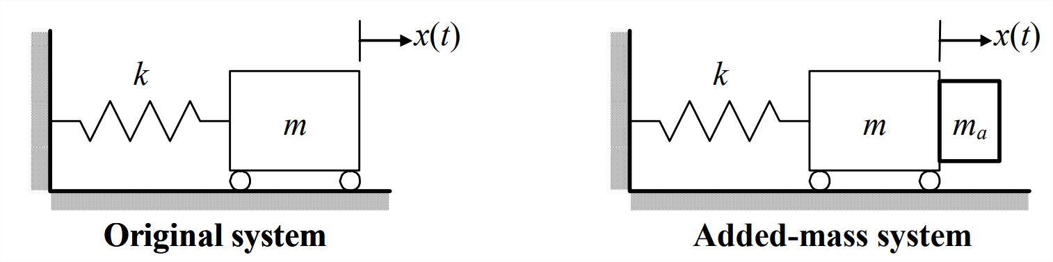
   Figure \(\PageIndex{9}\)

   1. Suppose that the parameters \(m\) and \(k\) of the original system are unknown, but that we know the value of the added mass \(m_{a}\), and that we are able to measure experimentally the natural frequencies \(\omega_{n}\) and \(\omega_{a n}\). Derive algebraically the following equation for the unknown mass \(m: \quad m=\frac{m_{a}}{\left(\omega_{n} / \omega_{a n}\right)^{2}-1}\). The traditional method described here may be called the added-mass or added-inertia method.⁶
   2. Apply the added-mass method of part 7.9.1 to calculate both the 2^nd order effective tipmass quantity \(m_E\) and the 2^nd order effective tip-stiffness constant \(k_{E}\) of the beam structural system shown on Figure 7.6.1. The data that you will need is stated in Example Problems 7.6.1 and 7.6.3: the measured natural frequency of the original system is \(f_{n}\) = 34.0 Hz; the concentrated-mass assembly that was added to the beam tip (Figure 7.6.5) weighs 0.254 lb; and the measured natural frequency of the added-mass system is \(f_{a n}\) = 15.85 Hz.
10. A distributed-parameter structural system⁷ is shown in the drawing; the “snapshot” of a dynamic deformation state (with exaggerated magnitude) is drawn in dashed lines. This system consists of an essentially rigid block of mass \(m\) and two parallel cantilever beams. The two flexible (in bending) beams are nominally uniform and identical to each other, with rectangular cross section of width \(b\), depth \(h\), and cross-sectional area \(A=b h\). The beams are embedded into the mass, just as they are embedded into the foundation below. In-plane rotation of mass \(m\) is suppressed by the very high axial stiffness of the beams and the separation of the two beams. The bending slopes of the beams where they join mass \(m\) are essentially zero due to the rigidity of mass \(m\) and of the beam-to-mass joints. Provided that forcing [such as \(f_{x}(t)\) on the drawing] and/or initial conditions are in the plane of the paper, motion of the mass is restricted to one-dimensional translation, \(x(t)\). You should be able to verify from a textbook on mechanics of materials that the total effective stiffness constant of the two beams that restrain motion of mass \(m\) is \(k_{E} \equiv\left(f_{x} / x\right)_{\text {static}}=2 \times 12 E I / L^{3}\). We can account for the contribution of the beams’ mass to the approximately 2^nd order dynamics of this system by using what is known in more advanced theory as the consistent mass of a distributed-parameter structure. We denote the weight per unit volume of the beam material as \(w\) and the mass as density \(\rho \equiv w / g\). Then the total consistent mass from the two beams, which effectively moves with mass \(m\) through translation \(x(t)\), is \(2 m_{c}=2 \times(156 / 420) \rho A L\) (Craig, 1981, page 387); thus, the total effective mass of the structural system is \(m_{E}=m+2 m_{c}\).

    

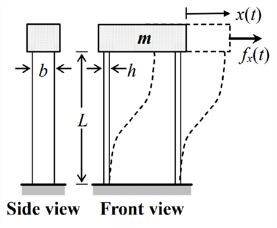
    Figure \(\PageIndex{10}\)

    1. Write an algebraic equation for the natural frequency \(\omega_{n}\) in rad/s of this structural system in terms of the system parameters \(E\), \(I\), \(L\), \(m\), \(w\), \(A\), and \(g\).
    2. Consider an actual fabricated version of this structural system, shown in the photograph, which is used in an instructional laboratory experiment⁸. The beams are extruded aluminum “flats”, from which students made the following careful measurements of average dimensions and properties: \(L\) = 12.00 inches, \(b\) = 2.010 inches, \(h\) = 0.1259 inch; \(w\) = 0.0965 lb/inch³; \(E\) = 9.40e+6 lb/inch². The relatively rigid mass \(m\) was machined from an aluminum block; the students measured its weight as 1.61 lb. Calculate the natural frequency \(f_{n}\) in Hz of this laboratory apparatus.

       

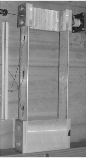
       Figure \(\PageIndex{11}\)

¹The same basic principles of dynamics and fluid statics apply if the vehicle is a submerged submarine.

²The \(LC\) circuit is a simplified model for devices such as antennas and cavity resonators that transmit and receive electromagnetic energy (Halliday and Resnick, 1960, Chapters 38 and 39). Also, cascades of \(LC\) pairs are often used as passive filters in radio-frequency, 100 kHz and above, applications (Horowitz and Hill, 1980, pages 654-656).

³This circuit with op-amps, capacitors, and resistors is essentially the electronic analog computer (see the footnote to Problem 5.6) for solving ODE 7.1.5.

⁴Example Problem 7.6.3 describes how tiny gaps between the thick steel clamping plates and the aluminum beam surfaces might change the effective beam length \(L\). It is worth observing also that another possible source of stiffness error, which is difficult to assess quantitatively, is some significant flexibility in the steel clamping plates. The theoretical equation for beam-tip stiffness is based on the assumption that the clamping medium is completely rigid.

⁵Propagation of error is discussed in textbooks on experimental instrumentation and measurements, for example, Dally, Riley, and McConnell, 1984, pages 544-545.

⁶The added-mass method is an elegantly simple technique for finding experimentally the unknown parameters of a 2^nd order, or approximately 2^nd order, linear mechanical system. The method requires only that we be able to measure accurately the free-vibration frequencies; otherwise, the motion sensors and other instrumentation can be uncalibrated. Use of the added-mass method is a simple example of system identification, which is discussed at greater length in Section 9.9.

⁷This structure is a rudimentary form of one-story shear building that is used for studying the structural dynamics of buildings (Craig, 1981, pages 42, 265, 346, etc.; Clough and Penzien, 1974, pages 226-227). The rigid mass represents a floor slab/girder, and the flexible beams represent structural columns.

⁸The principal plane of the actual laboratory apparatus is horizontal relative to gravity. The photograph is rotated 90° to make the plane appear vertical, in order to match the drawing on the previous page.