7.6: Introduction to Vibrations of Distributed-Parameter Systems

A system such as the mechanical mass-dashpot-spring system of Figure 7.1.1 is often called a lumped-parameter system. This descriptive term is used because the essential physical features are idealized to be spatially concentrated: in Figure 7.1.1, all of the mass is idealized to reside in one physical element, all of the damping in another, and all of the stiffness in yet another. Some engineering systems can be modeled accurately using idealized lumped elements; but many real systems cannot, and these latter are called distributed-parameter systems. A structural beam, such as that shown in Figure 7-6 on the next page, is a prototypical distributed-parameter mechanical system. It is obvious that the mass of this beam is not concentrated at a single point in space, but instead is distributed throughout the beam’s volume. Similarly, the flexibility of the beam does not reside in a discrete spring, but also is distributed over the entire spring. Finally, although there is very little damping in this particular system, it also is distributed throughout the beam in the forms of molecular “friction” within the deforming beam and fluid dynamic drag on the beam’s surface if the beam is immersed in air, another gas, or liquid.

Figure \(\PageIndex{1}\): Clamped uniform aluminum beam with nominal cross section 2 inch \(\times\) 81 inch. Test configuration: beam clamped at left between thick steel plates, leaving 10.0 inches of overhang; non-contacting proximity (displacement) sensor over right tip; bonded onto the beam’s right tip is a small, thin, steel plate, the “target” in which the proximity sensor induces eddy currents.

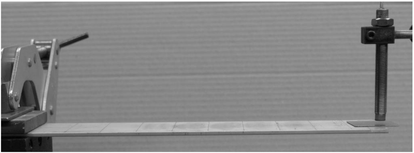
Figure \(\PageIndex{2}\) is an actual record of motion of the beam in Figure \(\PageIndex{1}\) in response to a particular initial condition: the tip of the beam was bent upward statically, then released¹.

Figure \(\PageIndex{2}\): Initial-translation dynamic response of the beam in Figure \(\PageIndex{1}\), as detected by the proximity sensor.

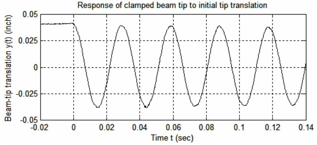
The subsequent time response was directly analogous to the theoretical IC response shown in Figure 7.3.1, with positive initial deflection, \(y_{0}>0\), but zero initial velocity, \(\dot{y}_{0}=0\), \(y(t)\) being vertical translation, positive upward, of the beam tip relative to the static equilibrium position under gravity loading. Note in Figure \(\PageIndex{2}\) that the character of the measured response appears very close to that predicted theoretically in Eq. (7-10) for an undamped 2^nd order system, \(y(t)=y_{0} \cos \omega_{n} t\). However, we can detect by detailed analysis of the data in Figure \(\PageIndex{2}\) the following very small differences between actual and theoretical responses:

1. (i) slight reductions in amplitude from one cycle to the next, due to the very light system damping and to an imperfect release of the beam from its static initial deformation;
2. (ii) a slight eccentricity of the vibration relative to the zero-translation position, due to a small instrumentation error, which is almost unavoidable in experimental measurements; and
3. (iii) almost imperceptibly small distortion of the waveform shape relative to a perfect cosine.

(More easily observed distortion appears in Figure \(\PageIndex{4}\), which is discussed below.) This small waveform distortion occurs because the beam is not a perfect 2^nd order, lumped-parameter system; in reality, the beam is, mathematically, a much more complicated distributed-parameter system. Nevertheless, it turns out that in many circumstances, including this particular one, we can approximately model distributed-parameter structures as 2^nd order systems, with acceptable accuracy for many engineering purposes.

Careful study of the experimental data in Figure \(\PageIndex{2}\) shows that the time between any two successive peaks of the response signal, the “period” of damped vibration, is \(T_{d}\approx\)0.029 4 s. The system of Figure \(\PageIndex{1}\) is damped, so \(T_d\) is not a true undamped “natural” period. However, theoretical solutions for mathematical models predict that a measured period such as this for a very lightly damped system is almost equal, for all practical purposes, to the true natural period. Therefore, in the example problems below, we shall assume that the measured period is the system's natural period, and so the undamped natural frequency is \(f_{n} \approx 1 / T_{d}=\) 34.0 Hz.

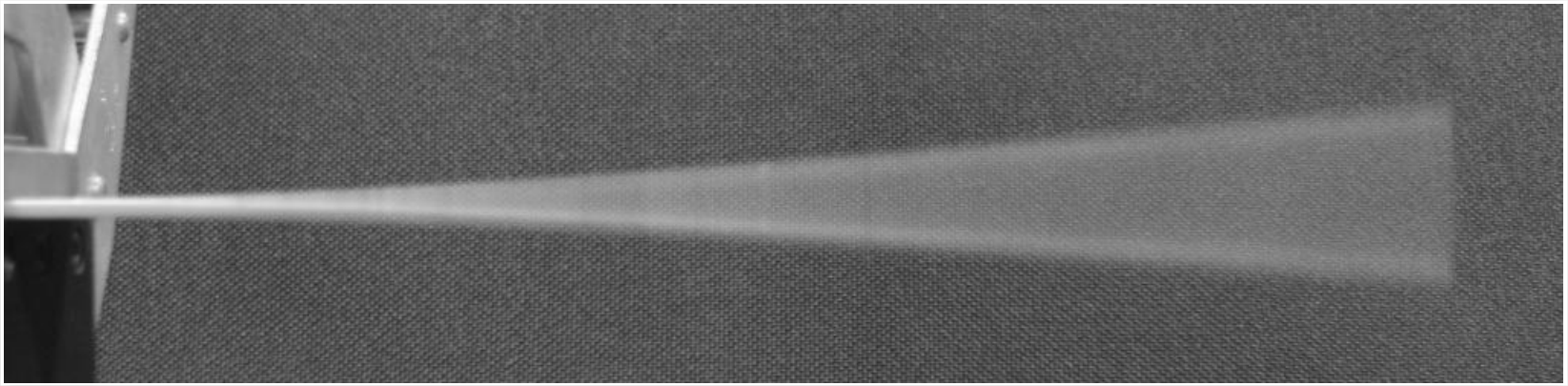
Figure \(\PageIndex{3}\) illustrates the spatial distribution of the beam vibrating after the same type of initial condition as that of Figure \(\PageIndex{2}\), but with a much greater magnitude of deformation. For this edge-on photo, the shutter of the digital camera was open for \(\frac{1}{4}\) second, during which time the beam vibrated through 8+ complete cycles. The upper and lower limits of dynamic deformation appear as fairly distinct curved lines against the dark background in the photo, whereas the intermediate states of deformation appear as a blur. This occurs because the velocity of motion was zero at the extreme deformations; therefore the digital camera’s photosites were exposed during disproportionately longer times to the extreme deformations than to the intermediate deformations.

Figure \(\PageIndex{3}\): Edge-on, \(\frac{1}{4}\)-second exposure photo of the beam of Figure \(\PageIndex{1}\) vibrating after an initial static deformation and release of the beam tip.

Example \(\PageIndex{1}\): A Calculation of the "Effective" Tip Mass of the Vibrating Beam

Consider the system of Figure \(\PageIndex{1}\). By loading the beam statically with small calibrated weights hanging from the beam tip, and by measuring the resulting beam-tip downward vertical deflection with the proximity sensor, students determined a beam-tip average “effective” stiffness constant to be \(k_{E}=7.86\) lb/inch. With this stiffness and the measured natural frequency \(f_{n}\) = 34.0 Hz, we can infer a value for the “effective” tip mass from Equation 7.1.3 in the form

\[m_{E}=\frac{k_{E}}{\omega_{n}^{2}}=\frac{k_{E}}{\left(2 \pi f_{n}\right)^{2}}=\frac{7.86 \mathrm{lb} / \mathrm{inch}}{\left(2 \pi \times 34.0 \mathrm{s}^{-1}\right)^{2}}=1.72 \mathrm{e}-4 \mathrm{lb}-\mathrm{s}^{2} / \mathrm{inch} \nonumber \]

It is appropriate to conduct a plausibility check of this result, especially since most of us find it difficult to relate intuitively to values of mass that are expressed in the traditional structural system of units (see Section 3-1). Students measured the 10.00-inch overhang of the uniform aluminum beam in Fig. 7-6 to weigh Wb = 0.230 lb, and they measured the weight of the small steel target at the beam tip as 0.13 oz = 0.0081 lb. Therefore, the total mass of the beam plus the target is

\[m_{T}=W_{T} / g=(0.238 \mathrm{lb}) \div\left(386.1 \mathrm{inch} / \mathrm{s}^{2}\right)=6.16 \mathrm{e}-4 \mathrm{lb}-\mathrm{s}^{2} / \mathrm{inch} \nonumber \]

The mass ratio is \(m_{E} / m_{T}\) = 0.28. In view of the photo of the vibrating beam, Figure \(\PageIndex{3}\), it seems physically plausible that roughly 28% of the total structural mass is effectively volved in the vibration. This ends Example Problem \(\PageIndex{1}\).

Example \(\PageIndex{2}\): Calculations Based Upon Ideal Theory, Normal DImensions, and Standard Material Constants

Let us calculate an estimate of the natural frequency of the beam system of Figure \(\PageIndex{1}\) using Equation 7.1.3 in the form \(f_{n}=\frac{1}{2 \pi} \sqrt{k_{E} / m_{E}}\). In this calculation, let us assume that we do not have measured data from actual hardware or instrumentation, i.e., that we have only the type of information that would normally be available in the preliminary-design phase of an engineering project, before even a prototype is fabricated.

Solution

First, let us calculate the theoretical effective stiffness constant \(k_E\). From your courses and textbooks on static structural behavior, you might be familiar with the deformation under loading of structural members such as uniform (prismatic) beams and shafts that are fabricated from homogeneous, isotropic, linearly elastic materials. The theory relevant to the present situation is that for a cantilever (ideally clamped-free) beam. From any textbook with the words “mechanics of materials” or “strength of materials” in its title², you can find that the effective stiffness at the tip of a uniform cantilever beam is \(k_{E}=3 E I / L^{3}\), in which \(E\) is the material modulus of elasticity, \(I\) is the 2^nd area moment (also called area moment of inertia) of the beam cross section, and \(L\) is the overhanging length of the beam. For the beam of Figure \(\PageIndex{1}\), let us use the standard (in preliminary-design calculations) elastic modulus for aluminum: \(E\) = 10.0e+6 lb/inch². The nominal rectangular cross-sectional dimensions of the beam are width \(b\) = 2.00 inches and depth \(h\) = 1/8 inch, for which the theoretical 2^nd area moment is \(I=b h^{3} / 12\) = 3.255e−4 inch⁴. Using the overhang length of 10.00 inches, we calculate the effective beam-tip stiffness to be

\[k_{E}=\frac{3 \times\left(10.00 \times 10^{6} \mathrm{lb} / \mathrm{inch}^{2}\right) \times\left(3.255 \times 10^{-4} \mathrm{inch}^{4}\right)}{(10.00 \mathrm{inch})^{3}}=9.766 \mathrm{lb} / \mathrm{inch} \nonumber \]

Next, let us calculate an effective tip mass \(m_{E}\). Consider first the vibration of an ideal uniform cantilever beam alone (i.e., without a concentrated tip mass such as the steel target shown on Figure \(\PageIndex{1}\)). More advanced theory³ shows that, for such a bare beam, the effective tip mass vibrating at the fundamental natural frequency is 0.242 672 of the total beam mass, which we determine next. The weight of a uniform beam is \(W_{b}=w A L\), in which \(w\) is the weight density (weight per unit volume), and the cross-sectional area of a rectangular beam is \(A=b h\). Let us use the standard (in preliminary-design calculations) weight density of aluminum, \(w\) = 0.1000 lb/inch³, so that the weight of our ideal cantilever beam is \(W_b\) = (0.1000 lb/inch³)\(\times\)(\(\frac{1}{4}\) inch²)\(\times\) 0.2500 lb. Hence, the effective tip mass of the bare beam alone is \(m_{b E}\) = (0.242 672 \(\times W_{b} / g\) = 0.242 672 \(\times\) (0.2500 lb) \(\div\) (386.1 inch/s²) = 1.571e−4 lb-s²/inch. To obtain an intuitively logical estimate of the total effective tip mass, we add to \(m_{b E}\) the mass of the steel target that is bonded to the beam tip on Figure \(\PageIndex{1}\): \(m_{E}=m_{b E}+(0.0081 \mathrm{lb}) \div\left(386.1 \mathrm{inch} / \mathrm{s}^{2}\right)=1.78 \mathrm{e}-4 \mathrm{lb}-\mathrm{s}^{2} / \mathrm{inch}\).

Finally, the natural frequency based upon ideal theory, nominal dimensions, and standard material constants is

\[f_{n}=\frac{1}{2 \pi} \sqrt{\frac{k_{E}}{m_{E}}}=\frac{1}{2 \pi} \sqrt{\frac{9.77 \mathrm{lb} / \mathrm{inch}}{1.78 \times 10^{-4} \mathrm{lb} \cdot \mathrm{s} ^{2} / \mathrm{inch}}}=37.3 \mathrm{Hz} \nonumber \]

See homework Problem 7.8 for an analysis of the discrepancy between this calculated natural frequency and the measured value of 34.0 Hz. This ends Example Problem 7-2.

The clamped-beam system of Figure \(\PageIndex{1}\) appears to behave very much like a 2^nd order system when it responds dynamically to a simple initial static deflection of the beam tip. However, when it is subjected to most other possible types of excitation, its dynamic response is more complicated. For example, when the beam tip was tapped lightly upward with a small hammer, the tip moved vertically as shown on Figure \(\PageIndex{4}\), next page.

Figure \(\PageIndex{4}\): Dynamic response to a hammer tap at time \(t\) = 0 s of the beam on Figure \(\PageIndex{1}\), as detected by the proximity sensor.

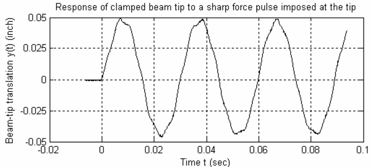
The input force that stimulated the response of Figure \(\PageIndex{4}\) was approximately a half-sine pulse (as described in Sections 1.5 and 1.6) of very short duration relative to the lightly damped period of this system, \(T_{d} \approx\) 0.029 4 s. In Chapter 8, theory is developed showing that, if the system were a true undamped 2^nd order system, then the time response to such a pulse would have almost a perfect sine waveform, starting at time \(t\) = 0 s. However, the waveform in Figure \(\PageIndex{4}\) is quite different from a perfect sine waveform; in fact, it is closer to being the sum of many sinusoids, in the general spirit of a Fourier series, but without the property of Fourier series that all higher series sinusoids have frequencies that are integer multiples of the frequency of the first (fundamental) sinusoid⁴. In the case of Figure \(\PageIndex{4}\), the total motion consists primarily of a first sinusoid with frequency 34.0 Hz, plus a second, lower-amplitude sinusoid with frequency approximately 215 Hz. The motion at 34.0 Hz represents the first (fundamental) mode of vibration, and the motion at 215 Hz represents the second mode of vibration.

In fact, the beam system of Figure \(\PageIndex{1}\) has many more than two modes of vibration, each with a characteristic frequency higher than that of the previous mode. The third and higher modes are not evident in Figure \(\PageIndex{4}\) only because the particular pulse stimulus applied in this case did not noticeably excite those higher modes; however, they could be excited by any number of other stimuli, such as sharp pulses applied at particular locations, high-frequency sound-pressure waves, etc. In reality, every distributed-parameter system is a higher-than-2^nd-order system, and, if only lightly to moderately damped, has many modes of vibration. For example, every acoustic musical instrument is a fluid or structural distributed-parameter system whose distinctive sound quality is a direct consequence of its particular modes of vibration⁵. However, except for this short descriptive introduction, the subject of distributed-parameter systems is beyond the scope of this book. The subject of vibration modes appears again in Chapter 12, which deals with undamped, 4^th order, lumped-parameter systems that have two modes of vibration.

Observe from Figure \(\PageIndex{4}\) that the translation response of the beam system of Figure \(\PageIndex{1}\) was still dominated by the first vibration mode, even though the tip-pulse stimulus also excited the second mode, but to a much lower amplitude than that of the first mode. Hereafter in this book, the only response of any distributed-parameter system that we shall consider is the contribution of the first mode, and we shall assume that it dominates the total response. Indeed, this is often a good engineering approximation for distributed parameter structural systems that include relatively large, spatially concentrated masses. Consider, for example, the system of Figure \(\PageIndex{5}\), which is the same as that of Figure \(\PageIndex{1}\) but with the addition at the beam tip of a concentrated-mass assembly that consists of two ceramic magnets and an aluminum spacer, and weighs 0.254 lb

Figure \(\PageIndex{5}\): Structural system of Figure \(\PageIndex{1}\), with the addition at the beam tip of two ceramic magnets and an aluminum spacer. Note the same steel-plate tip-target for the proximity sensor as on Figure \(\PageIndex{1}\).

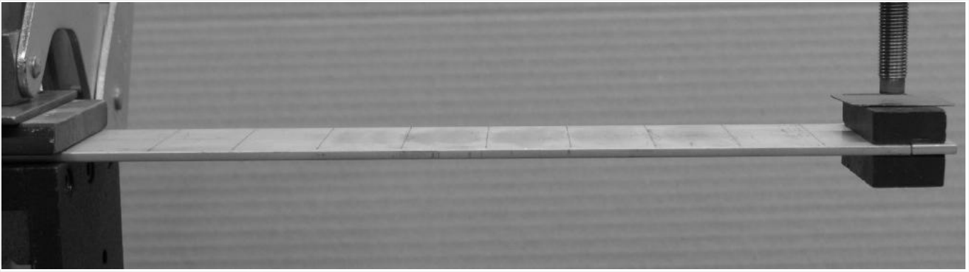
When the beam tip of Figure \(\PageIndex{5}\) was tapped lightly upward with a small hammer, the tip moved vertically as shown on Figure \(\PageIndex{6}\). The tip-translation response curve is a very clean sine waveform with almost no discernible distortion. The absence of significant distortion in the waveform means that, for our purposes, this beam-mass system behaves like a 2^nd order system, even though it is a distributed-parameter system.

Figure \(\PageIndex{6}\): Dynamic response to a hammer tap at time \(t\) = 0 sec of the beam on Figure \(\PageIndex{5}\), as detected by the proximity sensor.

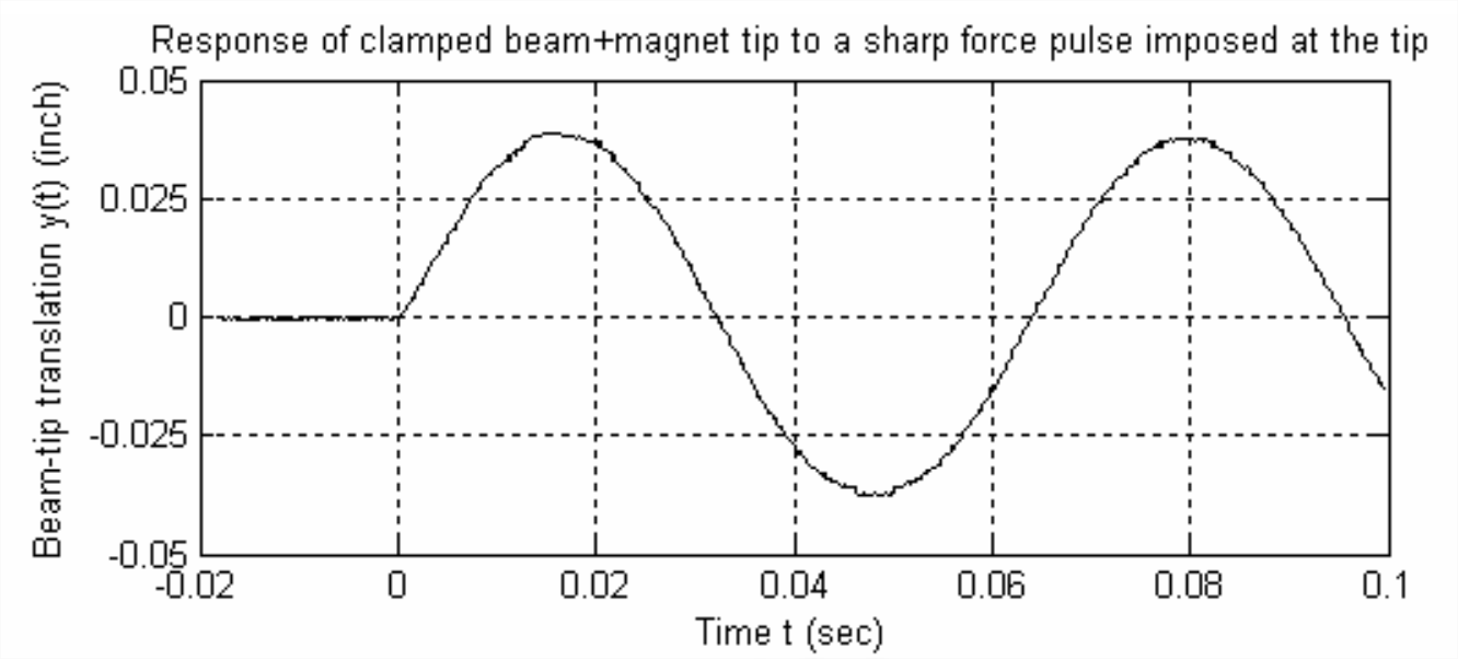
The addition of a relatively large quantity of mass at the beam tip reduces considerably the frequency of the waveform on Figure \(\PageIndex{6}\) relative to the 34.0-Hz frequency of the fundamental waveform on Figures \(\PageIndex{2}\) and \(\PageIndex{4}\); a careful analysis of the data in Figure \(\PageIndex{6}\) shows that the frequency of vibration is \(f\) = 15.85 Hz.

Example \(\PageIndex{3}\): a Predictive Calculation of the Vibrational Frequency of the Beam-Mass System of Figure \(\PageIndex{5}\)

Suppose that we had wanted to predict the frequency of the beam-mass system of Figure \(\PageIndex{5}\) before actually assembling the system and measuring the frequency. The following is an intuitively logical approach, though not necessarily theoretically rigorous. Providing that the clamped beam deforms linearly under load, the addition of mass and weight to the beam tip should not alter the beam’s stiffness constant, so we use the same measured beam-tip effective stiffness as that of Example Problem 7-1, \(k_E\) = 7.86 lb/inch. As stated previously, the concentrated-mass assembly that was added to the beam tip weighs 0.254 lb. To obtain the total effective vibrating tip mass, it seems reasonable to add together this value and the effective tip mass of the bare beam plus the steel target, as determined in Example Problem 7-1. Thus, we find the total effective mass \(m_E\) = 0.254 lb/(386.1 inch/s^2) + 1.72e−4 lb\(\cdot\)s²/inch = 8.30e−4 lb\(\cdot\)s²/inch. Finally, we calculate the predicted natural frequency to be

\[f_{n}=\frac{1}{2 \pi} \sqrt{\frac{k_{E}}{m_{E}}}=\frac{1}{2 \pi} \sqrt{\frac{7.86 \mathrm{lb} / \mathrm{inch}}{8.30 \times 10^{-4} \mathrm{lb} \cdot \mathrm{s} ^{2} / \mathrm{inch}}}=15.5 \mathrm{Hz} \nonumber \]

This predicted natural frequency is lower than the actual measured value of 15.85 Hz by a margin that is unexpectedly large, presuming that all assumptions underlying the theory are valid. This suggests that the actual effective stiffness during the dynamic response of Figure \(\PageIndex{6}\) was greater than 7.86 lb/inch. This is quite possible, because the students measured the beam-tip average effective stiffness constant to be 7.86 lb/inch over a range of very small downward deformation of the beam, but they also observed that the local stiffness (slope of the curve of load versus deflection) increased progressively as the downward deformation increased. Observe on Figures \(\PageIndex{1}\) and \(\PageIndex{5}\) at the clamped end of the beam that there appears to be a small gap between the edge of the upper steel clamping plate and the beam top surface; although not clearly visible on these photos, there is a similar gap between the lower clamping steel plate and the beam lower surface. These gaps are widest when the beam is undeformed, but as the beam is deformed downward, the lower gap gradually closes, thus slightly reducing the beam’s effective length \(L\) and thereby more significantly increasing its tip stiffness, \(k_{E}=3 E I / L^{3}\), from Example \(\PageIndex{2}\). The static gravity load of the concentrated-mass assembly shown on Figure \(\PageIndex{5}\) closed the lower gap, relative to its width on Figure \(\PageIndex{1}\) without the concentrated-mass assembly. Thus, it is indeed likely that the average beam-tip stiffness during the response recorded on Figure \(\PageIndex{6}\) was greater than that during the responses recorded on Figures \(\PageIndex{2}\) and \(\PageIndex{4}\). The actual clamping support and restraint of the aluminum beam in this experiment is clearly not the ideal, perfectly sharp edge and completely rigid wall that the elementary theory assumes for a cantilever beam.

¹In practice, this procedure is often called twang testing (also snapback, step-relaxation, and pluck testing)—see homework Problem 9.4 for a more detailed discussion.

²Examples of such textbooks, listed in the References section: Beer and Johnston, 1992; Hibbeler, 1997; and Timoshenko and Young, 1962.

³Theory from, among many possible sources, the following textbooks on structural dynamics that are listed in the References section: Bisplinghoff, et al., 1955, Example 3-1; Craig, 1981, Example 10.3; Meirovitch, 1967, Section 5-10; and Meirovitch, 2001, Example 8.4.

⁴The subject of Fourier series is developed in most textbooks on advanced calculus (for example, Hildebrand, 1962, pages 216-226) and in most textbooks on elementary partial differential equations.

⁵If you are interested in the physics of musical instruments, see Cannon, 1967, Sections 13.2-13.6, for an excellent introduction written by an engineer for students of engineering.