7.5: Dynamic Motion of a Mechanical System Relative to a Non-Trivial Static Equilibrium Position; Dynamic Free-Body Diagram

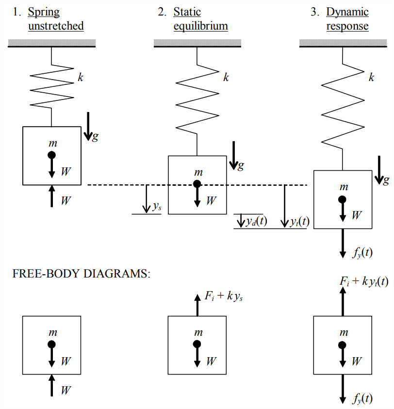
Consider the mass-spring system depicted in Figure \(\PageIndex{1}\) (on the next page), which is representative in many respects of some real mechanical systems. The system is oriented vertically in a gravity field with acceleration of gravity \(g\). Moreover, let us suppose that the spring is close-wound: a helical extension spring which, in its unstretched state, is wound with its coils forced into contact with each other, such that an initial tension force \(F_i\) is required to break the coil contact and allow the spring to begin stretching (Shigley and Mitchell, 1983, p. 449). Figure \(\PageIndex{1}\) illustrates three possible states of such a system. The weight of mass \(m \)is \(W=m g\), and it is a constant force vector acting downward through the center of gravity of the mass. The spring has stiffness constant \(k\) and initial tension \(F_i\), so that the spring law is \(f_{y}=F_{i}+k y\) for \(f_{y} \geq F_{i}\), where \(y\) is spring stretch vertically downward. State 1 of Figure \(\PageIndex{1}\) shows the mass supported statically by an externally applied force \(W\) acting upward, with the spring unstretched and therefore exerting no force on the mass. We define \(y_{t}(t)\) as the total vertical motion of the mass (positive downward in this example, but not necessarily always so) relative to the unstretched spring position. Now, if the externally applied upward force is slowly reduced, the weight of the mass is gradually transferred to the spring, and the spring stretches (provided that \(W>F_{i}\)), lowering the mass. State 2 of Figure \(\PageIndex{1}\) is the static equilibrium state that results after the externally applied upward force shrinks to zero, with the spring stretched by the amount \(y_{s}\) from the State 1 position. From the FBD of State 2, the equation of vertical static force equilibrium is

\[F_{i}+k y_{s}=W \quad \Rightarrow \quad y_{s}=\frac{W-F_{i}}{k}, \text { for } W \geq F_{i}\label{eqn:7.15} \]

State 3 of Figure \(\PageIndex{1}\) is a condition of dynamic response, with the dynamic force \(f_{y}(t)\) acting on the mass. We define the dynamic position \(y_{d}(t)\) as the motion relative to the static equilibrium position, \(y_{s}\) of Equation \(\ref{eqn:7.15}\). We see from Figure \(\PageIndex{1}\) that the total translation (from the unstretched-spring position) and the associated acceleration are

\[y_{t}(t)=y_{s}+y_{d}(t) \Rightarrow \ddot{y}_{t}(t)=\ddot{y}_{d}(t)\label{eqn:7.16} \]

The acceleration equation reflects the constancy of \(y_s\). Let us use the FBD for State 3 to write Newton’s 2^nd law for vertical translation:

\[\Sigma(\text { Forces })_{y}=m \ddot{y}_{t}=f_{y}(t)+W-\left(F_{i}+k y_{t}\right) \Rightarrow m \ddot{y}_{t}+k y_{t}=f_{y}(t)+W-F_{i}\label{eqn:7.17} \]

Now use Equation \(\ref{eqn:7.16}\) to eliminate \(y_{t}(t)\) from Equation \(\ref{eqn:7.17}\):

\[m \ddot{y}_{d}+k\left(y_{s}+y_{d}\right)=f_{y}(t)+W-F_{i}\label{eqn:7.18} \]

Next, eliminate \(k y_{s}=W-F_{i}\), Equation \(\ref{eqn:7.15}\), from Equation \(\ref{eqn:7.18}\) in order to express the ODE in terms of the motion relative to the static equilibrium position, the single dependent variable, \(y_{d}(t)\):

\[m \ddot{y}_{d}+k y_{d}=f_{y}(t)\label{eqn:7.19} \]

It is obvious physically that Equation \(\ref{eqn:7.19}\) is valid provided the upward dynamic motion does not exceed the static spring stretch: \(y_{t}(t)=y_{s}+y_{d}(t)>0\), i.e., \(y_{d}(t)>-y_s\).

Figure \(\PageIndex{1}\): Static and dynamic positions of a hanging, spring-supported weight

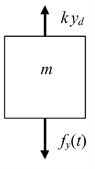
Equation \(\ref{eqn:7.19}\) is identical in form to Equation 7.1.2, which applies for a mass-spring system oriented horizontally, with no involvement of a close-wound spring or gravity. The only difference is that the unknown in Equation \(\ref{eqn:7.19}\) is not the total motion, but, instead, the motion relative to the static equilibrium position established by gravity and the spring initial tension. Consider the dynamic free-body diagram (DFBD) shown in Figure \(\PageIndex{2}\) on the next page, which is similar to that of State 3 in Figure \(\PageIndex{1}\), but without weight \(W\) and with only the spring force relative to the static equilibrium position. These changes from the FBD of State 3 in Figure \(\PageIndex{1}\) are equivalent to eliminating \(k y_{s}=W-F_{i}\) from Equation \(\ref{eqn:7.18}\) in order to obtain Equation \(\ref{eqn:7.19}\). Clearly, applying Newton’s 2^nd law to the DFBD Figure \(\PageIndex{2}\) leads again, and much more easily, to Equation \(\ref{eqn:7.19}\). The important conclusion here: if we want to solve only for the dynamic motion \(y_d(t)\) relative to the static equilibrium position, not the total motion relative to the springundeformed position, then we should use a DFBD from which all static influences (weight and spring initial tension in this case) have been eliminated. The DFBD should include only dynamic forces (and/or moments) relative to the static equilibrium position.

Figure \(\PageIndex{2}\): Dynamic freebody diagram

This conclusion is useful more generally because, in many situations, we are, indeed, interested primarily in the dynamic response relative to the static equilibrium position. Homework Problem 7.3 is one example. Moreover, this conclusion based upon the simple mass-spring system of Figure \(\PageIndex{1}\) has broad applicability to other mechanical systems. The subjects of Chapters 11 and 12 are more complex rotational systems and higher-order mechanical systems. It is usually convenient when analyzing those systems to deal only with the simpler DFBDs and ODEs that we use when we solve only for the dynamic motion relative to the static equilibrium position.

However, there are at least two classes of mechanical systems for which we must include (in FBDs and ODEs of motion) the weights of massive components:

1. pendulous systems for which gravity provides a spring effect, such as the simple pendulum example in Section 7.1 and the balloon-basket vehicle of homework Problem 7.4;
2. systems for which initial conditions and/or dynamic inputs (forces, moments) are defined relative to the undeformed-spring state, for example, the airplane landing contact of homework Problem 7.5.