15.2: Examples of P and PI Control

Figure \(\PageIndex{1}\) on the next page depicts a mechanical plant that is appropriate for the purpose of illustrating P control and PI control. A lightweight rotor is immersed in a viscous liquid, so that the damping moment imposed upon the rotor is \(-c_{\theta} \dot{\theta}\). The rotor is attached to the mechanical operator-setting device (a control wheel, for example) through a highly flexible torsion spring that has rotational stiffness constant \(k_{\theta}\). The rotor has sufficiently low rotational inertia \(J\), and viscous damping constantt \(c_{\theta}\) is sufficiently large, that we assume inertial moment \(-J \ddot{\theta}\) to be negligible in comparison with the damping and structural moments.

Figure \(\PageIndex{1}\): Lightweight rotor immersed in a viscous liquid, with connection to the input through a soft torsion spring. (Copyright; author via source)

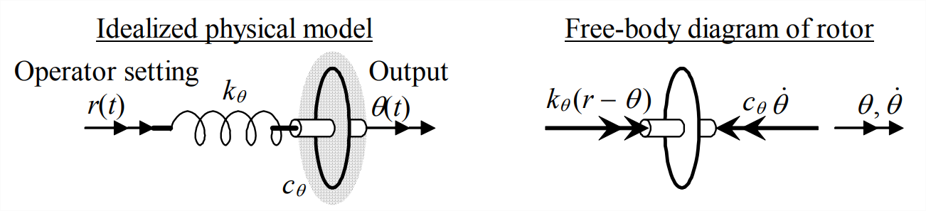
The equation of motion comes from the FBD on Figure \(\PageIndex{1}\):

\[k_{\theta}(r-\theta)-c_{\theta} \dot{\theta}=J \ddot{\theta} \approx 0 \Rightarrow \frac{c_{\theta}}{k_{\theta}} \dot{\theta}+\theta=r \Rightarrow \tau_{1} \dot{\theta}+\theta=r(t), \text { where } \tau_{1}=\frac{c_{\theta}}{k_{\theta}}\label{eqn:15.4} \]

Taking the Laplace transform of Equation \(\ref{eqn:15.4}\) gives the basic plant transfer function:

\[\operatorname{PTF}(s)=\frac{L[\theta(t)]}{L[r(t)]} \equiv \frac{\Theta(s)}{R(s)}=\frac{1}{\tau_{1} s+1}\label{eqn:15.5} \]

Clearly, this idealized open-loop mechanical plant by itself is a simple 1^st order system with time constant \(\tau_{1}=c_{\theta} / k_{\theta}\); furthermore, this system is the rotational equivalent of the translational series damper-spring low-pass filter described by Figure 3.7.4 and Equation 3.7.5.

The input to the plant is operator-setting angle \(r(t)\), and the output is rotor position \(\theta(t)\). From ODE Equation \(\ref{eqn:15.4}\), we see that the pseudo-static output is exactly equal to the input, \(\theta_{p s}(t)=r(t)\). So let us specify that our control objective for this system is to make the actual output \(\theta(t)\) be as close as possible to input \(r(t)\). To develop a physical feel for the behavior of the open-loop plant in Figure \(\PageIndex{1}\), let us suppose that the operator quickly moves the control wheel to one side so that input \(r(t)\) is close to a step function. The torsion spring will immediately be wound up more tightly, and will impose a moment upon the rotor. However, as we can visualize intuitively, the viscous restraint upon the rotor will prevent it from moving as quickly as the input, and the rotor angle will lag the input. As time goes on and the torsion spring gradually unwinds, the rotor angle will eventually settle to the input angle.

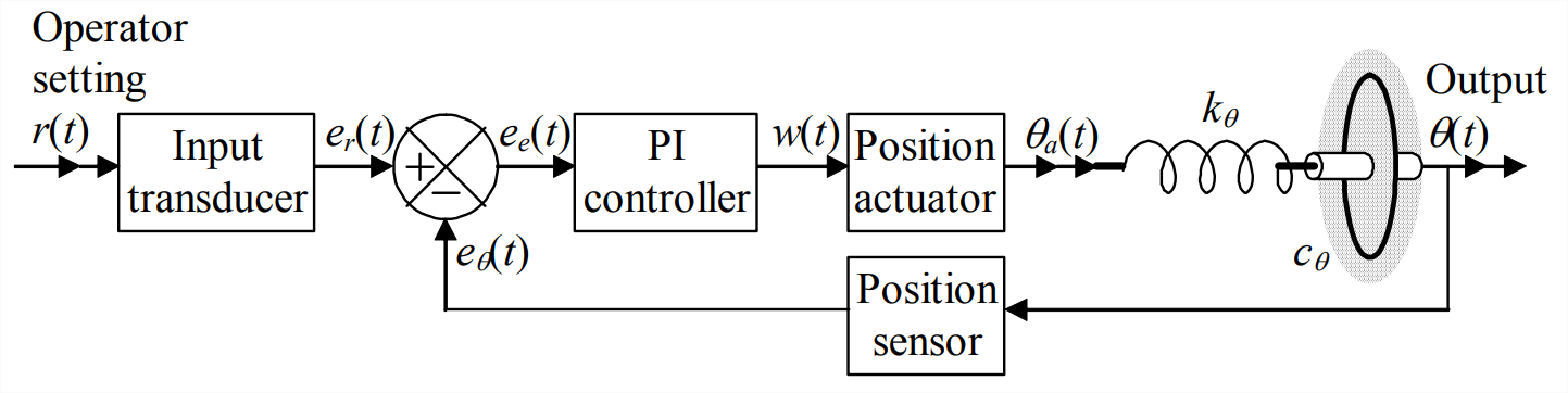
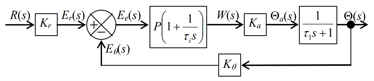
Let us suppose that the open-loop response is too slow for our purposes, and that we want to speed-up the response by using sensors, an actuator, feedback, and P or PI control in the system depicted on the next page, in functional form on Figure \(\PageIndex{2}\), and as a corresponding Laplace block diagram on Figure \(\PageIndex{3}\). The transfer function on Figure \(\PageIndex{3}\) for the P or PI controller comes from Equation 15.1.2, and the transfer function for the rotor-spring-liquid plant comes from Equation \(\ref{eqn:15.5}\). The input transducer and the output position sensor shown on Figures \(\PageIndex{2}\) and \(\PageIndex{3}\) are familiar from Chapter 14 (on Figure 14.3.1, for example). But the “position actuator” is something new. Whereas the output of most motors is torque, the output of this position actuator is specified to be rotational position. To make an actuator behave in this manner requires a feedback control system within the actuator itself; this is a characteristic of control systems that we now pause to examine.

Figure \(\PageIndex{2}\): Functional diagram of a system for controlling the position of a spring-connected rotor in a viscous liquid, based on proportional-integral control. (Copyright; author via source)

Figure \(\PageIndex{3}\): Laplace block diagram of a system for controlling the position of a spring-connected rotor in a viscous liquid, based on proportional-integral. (Copyright; author via source)

In fact, most actuators and sensors of all types are themselves complicated dynamic systems, often with internal feedback circuits. But this begs the following question: if there are control systems within actuators and/or sensors, then why are not the details of these systems included in the device or sub-system transfer functions shown on block diagrams such as Figure \(\PageIndex{3}\)?

A general response to this question is based upon the relative “speeds” of different systems. To illustrate this concept of system speed, we imagine that two standard 2^nd order systems, A and B, have equivalent values of subcritical viscous damping ratio \(\zeta\), but that System A’s undamped natural frequency is 100 times that of System B, \(\omega_{n A} / \omega_{n B} = 100\). Consequently, System A’s settling time for step inputs, \(t_{s A}=4 /\left(\zeta \omega_{n A}\right)\) [Equation 9.8.11], is only 0.01 that of System B; in this case, we regard “the dynamics of System A” as being “100 times faster” than “the dynamics of System B.” Engineers usually select for a control system sensors¹ and, when possible, actuators that are much faster than the dynamics of the plant under control; in such cases, we usually approximate the behavior of a sensor or actuator with a simple linear sensitivity constant, in equations such as \(e_{r}(t)=K_{r} r(t)\), \(e_{\theta}(t)=K_{\theta} \theta(t)\), and \(\theta_{a}(t)=K_{a} w(t)\), all of which are represented on Figure \(\PageIndex{3}\). In these cases, we are making the approximation that the dynamics of the sensors and actuators are essentially infinitely fast and are independent of, or “uncoupled from” the dynamics of the plant.

Be aware, though, that the full dynamics of devices used for control, especially actuators, cannot always be considered uncoupled from the dynamics of the plant. For one example, the dynamics of a reaction-mass actuator (homework Problem 10.15) in a vibration-control system are usually inextricably coupled with those of the structural plant, as in homework Problem 12.6. For another example, homework Problem 15.7 is an exercise of incorporating the dynamics of a position actuator into a control-system model; in this case, the process involves even more than just inserting the actuator’s transfer function in series within the block diagram of the overall system. In yet another example, Dettmer, 1995, Section 1.3.4 describes a control system for which it was necessary to account for the dynamic characteristics of both sensors and actuators.

Returning now to the rotor-position control system of Figures \(\PageIndex{2}\) and \(\PageIndex{3}\), our objective is to make the output follow the input, \(\theta(t) \approx r(t)\), so it is appropriate to define a revised (relative to Figure \(\PageIndex{1}\)) open-loop configuration. If the feedback loop in Fig. 15- 5 were broken, and if the PI controller were not present (\(P\) = 1, \(b_i\) = 0), then the transfer function for this open-loop system clearly would be \(K_{r} \times K_{a} \times 1 /\left(\tau_{1} s+1\right)\). We want this to be the same as that of the bare (devoid of control devices) plant, Equation \(\ref{eqn:15.5}\), so let us suppose that we have the ability to set the sensitivities of the input transducer and the position actuator so that \(K_{r} \times K_{a}=1\). Also, it will greatly simplify the algebra in the following developments if we suppose further that we can use identical sensors on the input angle and the output angle in the feedback path, so that \(K_{r}=K_{\theta}\). To summarize, we shall apply the following restrictions on the device sensitivities:

\[K_{r} \times K_{a}=1 \quad \text { and } \quad \frac{K_{\theta}}{K_{r}}=1\label{eqn:15.6} \]

To compare open-loop and closed-loop system performances, let us consider response (from zero initial conditions) to step input \(r(t)=R_{H} H(t) \Rightarrow R(s)=R_{H} / s\). Then, for the open-loop system, using transfer function Equation \(\ref{eqn:15.5}\) and partial-fraction expansion gives

\[\Theta(s)=R_{H} \frac{1}{s} \frac{1}{\tau_{1} s+1}=R_{H}\left(\frac{1}{s}-\frac{1}{s+1 / \tau_{1}}\right)\label{eqn:15.7} \]

Taking the inverse Laplace transform gives the step response of the open-loop system:

\[\theta(t)=R_{H}\left(1-e^{-t / \tau_{1}}\right), \text { for } t \geq 0\label{eqn:15.8} \]

Equation \(\ref{eqn:15.8}\) is simple 1^st order step response of the type shown on Figure 3.4.2. At the end of this section, there is a comparative numerical evaluation of this open-loop response and step responses for P and PI types of closed-loop control. For now, though, let us just observe from Equation \(\ref{eqn:15.8}\) that the asymptotic or “final” value of response for times much greater than time constant \(\tau_{1}\) equals the magnitude of the step input, as required:

\[\lim _{t \rightarrow \infty} \theta(t)=R_{H}\label{eqn:15.9} \]

Next, let us analyze closed-loop proportional (P) control, for which \(b_{i}=0\) on Figure \(\PageIndex{3}\). Thus, for the closed loop on Figure \(\PageIndex{3}\), we have for Equation 14.4.6 the polynomials \(N_{G}=P \times K_{a}\), \(D_{G}=\tau_{1} s+1\), \(N_{H}=K_{\theta}\), and \(D_{H}=1\), which we use to find the following \(CLTF(s)\):

\[\frac{\Theta(s)}{R(s)}=K_{r} \times \frac{N_{G} D_{H}}{D_{G} D_{H}+N_{G} N_{H}}=\frac{K_{r} P K_{a}}{\tau_{1} s+1+P K_{a} K_{\theta}}=K_{r} K_{a} \frac{P}{\tau_{1} s+1+K_{r} K_{a} \frac{K_{\theta}}{K_{r}} P} \nonumber \]

With simplifying assumptions Equation \(\ref{eqn:15.6}\), this becomes

\[C L T F(s)=\frac{\Theta(s)}{R(s)}=\frac{P}{\tau_{1} s+1+P}=\frac{P}{1+P} \frac{1}{\left(\frac{\tau_{1}}{1+P}\right) s+1} \equiv \frac{P}{1+P} \frac{1}{\tau_{1 P} s+1}\label{eqn:15.10} \]

in which the new time constant for the proportionally controlled system is

\[\tau_{1 P} \equiv \frac{\tau_{1}}{1+P}\label{eqn:15.11} \]

For step input \(r(t)=R_{H} H(t) \Rightarrow R(s)=R_{H} / s\), Equation \(\ref{eqn:15.10}\) gives the transform

\[\Theta(s)=\frac{R_{H}}{s} \times C L T F(s)=R_{H} \frac{P}{1+P} \times \frac{1}{s} \frac{1}{\tau_{1 P} s+1}\label{eqn:15.12} \]

Hence, we find the step response of the proportionally controlled system just by comparing Equation \(\ref{eqn:15.12}\) with Equation \(\ref{eqn:15.7}\) and then modifying Equation \(\ref{eqn:15.8}\) appropriately:

\[\theta(t)=R_{H} \frac{P}{1+P}\left(1-e^{-t / \tau_{1} p}\right), \text { for } t \geq 0\label{eqn:15.13} \]

The asymptotic or “final” value of proportionally controlled step response for times much greater than time constant \(\tau_{1 P}\) is:

\[\lim _{t \rightarrow \infty} \theta(t)=R_{H} \frac{P}{1+P}\label{eqn:15.14} \]

This situation provides the opportunity to introduce the final-value theorem and to illustrate its application; this is a useful mathematical tool that is derived in the next section. This theorem allows us to find the finite asymptotic value of a time function \(f(t)\), assuming that such a value exists, based only on the Laplace transform \(L[f(t)]=F(s)\), without requiring that the equation for \(f(t)\) be available:

\[\lim _{t \rightarrow \infty} f(t)=\lim _{s \rightarrow 0}[s F(s)]\label{eqn:15.15} \]

For step response of the proportionally controlled system, the final-value theorem and Equation \(\ref{eqn:15.12}\) give

\[\lim _{t \rightarrow \infty} \theta(t)=\lim _{s \rightarrow 0} s \times \Theta(s)=\lim _{s \rightarrow 0}\left(s \times R_{H} \frac{P}{1+P} \frac{1}{s} \frac{1}{\tau_{1 P} s+1}\right)=\lim _{s \rightarrow 0}\left(R_{H} \frac{P}{1+P} \frac{1}{\tau_{1 P} s+1}\right)=R_{H} \frac{P}{1+P} \nonumber \]

This is another, easier method for finding result Equation \(\ref{eqn:15.14}\). The final-value theorem was not needed to derive the correct asymptotic solution for this simple case, but it will be a useful, labor-saving tool for more complicated cases in the future.

Comparing Equation \(\ref{eqn:15.14}\) with the required asymptotic value \(\lim _{t \rightarrow \infty} \theta(t)=R_{H}\), Equation \(\ref{eqn:15.9}\), we see that, because \(P /(1+P) \neq 1\), the proportionally controlled system fails to satisfy the requirement exactly. Let us examine possible values of proportional gain \(P\). Equation \(\ref{eqn:15.11}\) requires that \(P>-1\) so that the system is stable, \(\tau_{1 P}>0\). Equation \(\ref{eqn:15.13}\) requires that \(P > 0\) so that the response has the same sign as the input. Moreover, \(P\) should be a positive number as large as possible, within practical hardware limitations, because

1. the greater the value of \(P\), the smaller is time constant \(\tau_{1 P}\), making the system faster than the open-loop system, and
2. the greater the value of \(P\), the closer is the asymptotic value of the output to the value of the input, from Equation \(\ref{eqn:15.14}\).

The value \(P = 4\) is a commonly used proportional gain. But even for a large, positive value of \(P\), the steady-state response will be at least a little smaller than the input. The steady-state output error, also known as offset, is defined as

\[\Delta \theta_{\text {offeet}} \equiv R_{H}-R_{H} \frac{P}{1+P}=\frac{R_{H}}{1+P}\label{eqn:15.16} \]

A large value, \(P > 9\), is required to reduce the offset to less than 10% of the desired steady-state output.

There is a simple explanation for the offset produced by proportional (P) control, which also will suggest a remedy. Block diagrams Figure \(\PageIndex{2}\) and Figure \(\PageIndex{3}\) show that the final value of \(\theta_{a}\) must be non-zero, equal to the final value of output \(\theta\). In other words, the torsion spring must be completely relaxed (unloaded) at the end of the control process, which is obvious physically. Furthermore, by tracing backwards on the forward branches of the loops on Figures \(\PageIndex{2}\) and \(\PageIndex{3}\), we find the other relevant final values: \(w=\theta_{a} / K_{a}=\theta / K_{a}\), and, with \(b_{i}=0\), \(e_{e}=w / P=\theta_{a} /\left(K_{a} P\right)=\theta /\left(K_{a} P\right) \neq 0\). Ideally, the final error signal \(e_{e}=e_{r}-e_{\theta}\) should be zero, corresponding to the output being exactly the desired final value; however, the preceding argument shows that the final error for P control alone is inevitably non-zero. This argument also suggests that we seek some way to make the final error equal zero, \(e_{e}=0\), but still to preserve non-zero input into the position actuator, \(w \neq 0\), so that \(\theta_{a} \neq 0\), and so that the final output equals the desired value, \(\theta=r\). Integral (I) action can produce this effect: if we add a term to \(w\) that is proportional to the integral of the error signal, \(\int_{\tau=0}^{\tau=t} e_{e}(\tau) d \tau\), then we can have a final non-zero control signal, \(w \neq 0\), even though the final error itself is zero, \(e_{e}=0\).

Therefore, let us next find the closed-loop transfer function for closed-loop proportional-integral (PI) control (\(b_{i}=1\)). For the closed loop on Figure \(\PageIndex{3}\), the forward-branch transfer function is \(G=P\left(1+\frac{1}{\tau_{i} s}\right) \times K_{a} \times \frac{1}{\tau_{1} s+1}=\frac{P K_{a}\left(\tau_{i} s+1\right)}{\tau_{i} s\left(\tau_{1} s+1\right)}\), so \(N_{G}=P K_{a}\left(\tau_{i} s+1\right)\) and \(D_{G}=\tau_{i} s\left(\tau_{1} s+1\right)\). For the feedback branch, \(N_{H}=K_{\theta}\) and \(D_{H}=1\). Therefore, Equation 14.4.6 gives the following \(CLTF(s)\)):

\[\begin{aligned}
\frac{\Theta(s)}{R(s)} &=K_{r} \times \frac{N_{G} D_{H}}{D_{G} D_{H}+N_{G} N_{H}}=\frac{K_{r} P K_{a}\left(\tau_{i} s+1\right)}{\tau_{i} s\left(\tau_{1} s+1\right)+P K_{a}\left(\tau_{i} s+1\right) K_{\theta}} \\
&=K_{r} K_{a} \frac{P\left(\tau_{i} s+1\right)}{\tau_{i} s\left(\tau_{1} s+1\right)+K_{r} K_{a} \frac{K_{\theta}}{K_{r}} P\left(\tau_{i} s+1\right)}
\end{aligned} \nonumber \]

With simplifying assumptions Equation \(\ref{eqn:15.6}\), this becomes

\[\frac{\Theta(s)}{R(s)}=\frac{P\left(\tau_{i} s+1\right)}{\tau_{i} s\left(\tau_{1} s+1\right)+P\left(\tau_{i} s+1\right)}=\frac{P\left(\tau_{i} s+1\right)}{\tau_{i} \tau_{1} s^{2}+(1+P) \tau_{i} s+P}\label{eqn:15.17} \]

Before analyzing Equation \(\ref{eqn:15.17}\) in more detail, let us first determine if, as predicted above, PI control eliminates the P-control offset of Equation \(\ref{eqn:15.16}\). For step input \(r(t)=R_{H} H(t) \Rightarrow R(s)=R_{H} / s\), Equation \(\ref{eqn:15.17}\) gives the transform

\[\Theta(s)=\frac{R_{H}}{s} \frac{P\left(\tau_{i} s+1\right)}{\tau_{i} s\left(\tau_{1} s+1\right)+P\left(\tau_{i} s+1\right)}\label{eqn:15.18} \]

Applying final-value theorem Equation \(\ref{eqn:15.15}\) to Equation \(\ref{eqn:15.18}\) gives

\[\lim _{t \rightarrow \infty} \theta(t)=\lim _{s \rightarrow 0} s \times \Theta(s)=\lim _{s \rightarrow 0}\left(\frac{R_{H} P\left(\tau_{i} s+1\right)}{\tau_{i} s\left(\tau_{1} s+1\right)+P\left(\tau_{i} s+1\right)}\right)=\lim _{s \rightarrow 0}\left(R_{H} \frac{P}{P}\right)=R_{H}\label{eqn:15.19} \]

Therefore, integral action does indeed eliminate the error that is inevitable from purely proportional control.

Returning to transfer function Equation \(\ref{eqn:15.17}\), we see that integral action has increased the order of the system to 2^nd order from the 1^st order of the plant. Accordingly, we can re-write the transfer function in terms of parameters appropriate for a 2^nd order system:

\[\frac{\Theta(s)}{R(s)}=\frac{\frac{P}{\tau_{i} \tau_{1}}\left(\tau_{i} s+1\right)}{s^{2}+\frac{1+P}{\tau_{1}} s+\frac{P}{\tau_{i} \tau_{1}}} \equiv \frac{\omega_{n}^{2}\left(\tau_{i} s+1\right)}{s^{2}+2 \zeta \omega_{n} s+\omega_{n}^{2}}\label{eqn:15.20} \]

in which the undamped natural frequency and the viscous damping ratio are, respectively,

\[\omega_{n}=\sqrt{\frac{P}{\tau_{i} \tau_{1}}} \text { and } \zeta=\frac{1}{2 \omega_{n}} \frac{1+P}{\tau_{1}}=\frac{1}{2} \sqrt{\frac{\tau_{i}}{\tau_{1}}} \frac{1+P}{\sqrt{P}}\label{eqn:15.21} \]

Note that this system is not a standard 2^nd order system, as defined in Equation 9.2.2. The term \(\omega_{n}^{2} \tau_{i} s\) in the numerator of Equation \(\ref{eqn:15.20}\) makes this system non-standard; that term corresponds to right-hand-side dynamics in the ODE describing the system, which is \(\ddot{\theta}+2 \zeta \omega_{n} \dot{\theta}+\omega_{n}^{2} \theta=\omega_{n}^{2}\left(\tau_{i} \dot{r}+r\right)\). The non-standard character means, among other things, that the step-response specifications derived in Section 9.8 do not apply exactly for this system.

For comparison with the previous cases of open-loop and P control, let us solve for response of the PI-controlled system to step input \(r(t)=R_{H} H(t) \Rightarrow R(s)=R_{H} / s\). Equation \(\ref{eqn:15.20}\) gives the transform

\[\Theta(s)=\frac{R_{H}}{s} \frac{\omega_{n}^{2}\left(\tau_{i} s+1\right)}{s^{2}+2 \zeta \omega_{n} s+\omega_{n}^{2}}=R_{H}\left[\frac{\omega_{n}^{2} \tau_{i}}{\omega_{d}} \frac{\omega_{d}}{\left(s+\zeta \omega_{n}\right)^{2}+\omega_{d}^{2}}+\frac{1}{s} \frac{\omega_{n}^{2}}{\left(s+\zeta \omega_{n}\right)^{2}+\omega_{d}^{2}}\right]\label{eqn:15.22} \]

The second form of Equation \(\ref{eqn:15.22}\) is written subject to the condition \(|\zeta|<1\), so that \(\omega_{d}^{2} \equiv\omega_{n}^{2}\left(1-\zeta^{2}\right)>0\); since \(\zeta>0\) from Equation \(\ref{eqn:15.21}\), this means that we assume the system to be underdamped, at least initially. With Equation \(\ref{eqn:15.22}\) in the second form, we can apply the following inverse Laplace transforms. First, Equations 9.3.5, 9.3.8, and 9.3.9 give:

\[L^{-1}\left[\frac{\omega_{d}}{\left(s+\zeta \omega_{n}\right)^{2}+\omega_{d}^{2}}\right]=e^{-\zeta \omega_{n} t} \sin \omega_{d} t\label{eqn:15.23} \]

Next, Equations 9.3.5 and 9.6.5 give (see homework Problem 9.12):

\[L^{-1}\left[\frac{1}{s} \frac{\omega_{n}^{2}}{\left(s+\zeta \omega_{n}\right)^{2}+\omega_{d}^{2}}\right]=1-e^{-\zeta \omega_{n} t}\left(\cos \omega_{d} t+\frac{\zeta \omega_{n}}{\omega_{d}} \sin \omega_{d} t\right)\label{eqn:15.24} \]

Substituting Equation \(\ref{eqn:15.23}\) and Equation \(\ref{eqn:15.24}\) into the inverse transform of Equation \(\ref{eqn:15.22}\), then combining terms appropriately, gives the step response of the PI-controlled underdamped system:

\[\theta(t)=R_{H}\left[1-e^{-\zeta \omega_{n} t}\left(\cos \omega_{d} t+\frac{\zeta \omega_{n}-\omega_{n}^{2} \tau_{i}}{\omega_{d}} \sin \omega_{d} t\right)\right], \text { for } 0 \leq \zeta<1 \text { and } 0 \leq t\label{eqn:15.25} \]

In the numerical example to follow, we shall encounter cases of both underdamping and overdamping; therefore, it is appropriate to apply conversion Equation 9.10.2 to underdamped response equation Equation \(\ref{eqn:15.25}\) in order to write the following equation for step response of the PI-controlled overdamped system:

\[\theta(t)=R_{H}\left[1-e^{-\zeta \omega_{n} t}\left(\cosh \mu_{d} t+\frac{\zeta \omega_{n}-\omega_{n}^{2} \tau_{i}}{\mu_{d}} \sinh \mu_{d} t\right)\right], \text { for } 1<\zeta \text { and } 0 \leq t\label{eqn:15.26} \]

in which \(\mu_{d}=\omega_{d} \sqrt{\zeta^{2}-1}\).

Now that we have derived the equations for step response, let us evaluate a numerical case with physically plausible parameters; in particular, let us calculate and compare the step responses: Equation \(\ref{eqn:15.8}\) for the open-loop system; Equation \(\ref{eqn:15.13}\) for the P-controlled system; and Equation \(\ref{eqn:15.25}\) or Equation \(\ref{eqn:15.26}\) for the PI-controlled system. We let the time constant of the open-loop system have the value \(c_{\theta} / k_{\theta} \equiv \tau_{1}=1\) s, and we use the typical value \(P = 4\) for the proportional gain. For the PI-controlled system, we consider three different integral time constants, \(\tau_{i}=\) 1/3, 2/3, and 1 s. The following is a MATLAB M-file that calculates the step responses and plots them on a single graph:

%MATLABdemo151.m

%1st order system: spring-connected rotor in a viscous fluid

%Step responses: open-loop, P-controlled, and PI-controlled

t=0:.01:4;

tau1=1;%time constant of open-loop system = 1 sec

thOL=1-exp(-t/tau1);%open-loop step response ratio

P=4;tau1P=tau1/(1+P);

thP=P/(1+P)*(1-exp(-t/tau1P));%step response ratio, P control

plot(t,thOL,t,thP),hold

taui=[1/3 2/3 1];%step response ratios, three cases of PI control

for ni=1:3,

wn=sqrt(P/(taui(ni)*tau1));zeta=(1+P)/(2*wn*tau1);

sig=zeta*wn;case_taui_zeta=[ni taui(ni) zeta]

if zeta < 1

wd=wn*sqrt(1-zeta^2);

thPI(ni,:)=1-exp(-sig*t).*(cos(wd*t)+(sig-wn^2*taui(ni))/wd*sin(wd*t));

else

md=wn*sqrt(zeta^2-1);

thPI(ni,:)=1-exp(-sig*t).*(cosh(md*t)+(sig-wn^2*taui(ni))/md*sinh(md*t));

end

plot(t,thPI(ni,:),'k')

end

grid,xlabel('Time t (sec)'),ylabel('Step response ratio \theta(t)/R_H')

title('Position control of a spring-connected rotor in a viscous fluid')

The MATLAB command and resulting output are printed below. The three cases shown are for PI control with integral time constant (“taui”) \(\tau_i\) = 1/3, 2/3, and 1 sec; note the values of viscous damping ratio (“zeta”) \(\zeta\): the system is underdamped for \(\tau_i\) = 1/3 s, but overdamped for \(\tau_i\) = 2/3 and 1 s.

>> MATLABdemo151

Current plot held

case_taui_zeta =

1.0000 0.3333 0.7217

case_taui_zeta =

2.0000 0.6667 1.0206

case_taui_zeta =

3.0000 1.0000 1.2500

Figure \(\PageIndex{4}\) is the graphical output from the MATLAB M-file.

Figure \(\PageIndex{4}\): Step responses for no control (open-loop), proportional (P) control, and proportional-integral (PI) control. (Copyright; author via source)

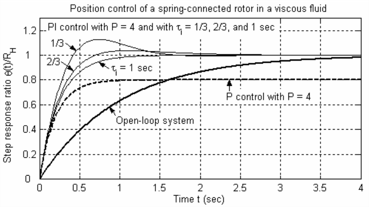
Figure \(\PageIndex{4}\) illustrates clearly the results derived previously regarding the time constants for open-loop and P control, and the final values of step response for open-loop, P control and PI control. The new and interesting results on Figure \(\PageIndex{4}\) relate to step response of the system under PI control. For all three values of \(\tau_{i}\), the speed of response is much faster than that of the open-loop system, and comparable to that for P control. Moreover, there is a design trade-off for this 2^nd order system between rise time and overshoot. Recall from Section 9.8 that rise time is the time required for the response first to reach the desired value, and overshoot is the maximum amount by which the response exceeds the desired value. For most cases, the control designer would like to make rise time as fast as possible, and to minimize overshoot. However, Figure \(\PageIndex{4}\) shows that we cannot simultaneously do both in this case: rise time is fastest for small \(\tau_{i}\), but overshoot is minimized or eliminated with larger \(\tau_{i}\). Therefore, the control designer must compromise and select a value of \(\tau_{i}\) that produces practically acceptable values of both rise time and overshoot, even though neither response parameter would be the best possible.

It is interesting to observe also from Figure \(\PageIndex{4}\) that, for this non-standard 2^nd order system, there is overshoot for \(\tau_{i}\) = 2/3 s \(\Rightarrow \zeta\) = 1.02; in other words, there is overshoot even though the system is overdamped. This is different from the step response of a positively damped standard 2^nd order system (Section 9.8), for which overshoot can occur only if \(0 \leq \zeta<1\).

¹Examples that appear in this book of such sensors are the accelerometer [homework Problem 10.12.2], the rate gyroscope (Example 9.2.2 in Section 9.2, and homework Problem 9.18), and the rate-integrating gyroscope (homework Problem 9.19).