15.1: Initial Definitions and PID Control

Figure \(\PageIndex{1}\) is a general functional block diagram that represents many engineering control systems. The term input-error operation can be defined in the context of this diagram: a single output quantity is fed back and differenced from the operator-setting input quantity, and the error signal is manipulated mathematically by a controller, also called control processor or filter, in such a way as to produce effective control. The controller usually consists of analog electronic circuitry and/or a digital processor.

Figure \(\PageIndex{1}\): Functional block diagram of general control system using input-error operations. (Copyright; author via source)

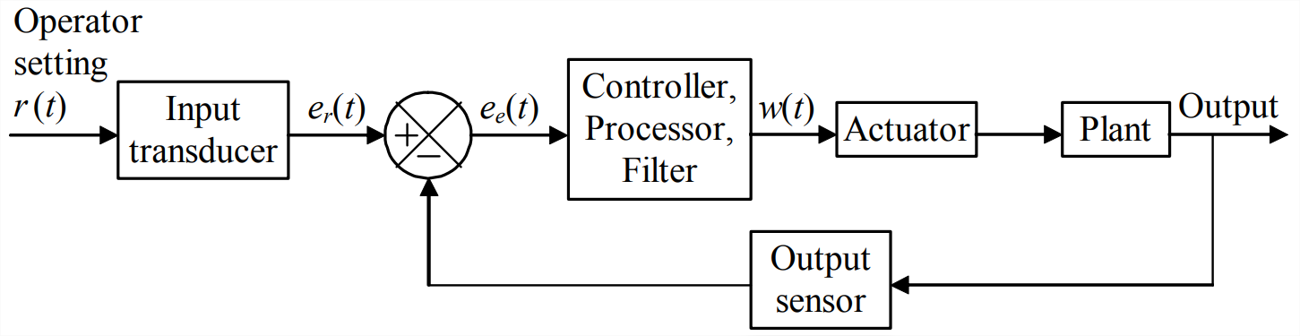
Proportional-integral-derivative (PID) control is a class of input-error operations used widely in industry. Let \(e_{e}(t)\) be the error voltage signal that is input to the controller and \(w(t)\) be the output voltage from the controller, as shown on Figure \(\PageIndex{1}\). The mathematical operations performed by an ideal PID controller are described by the equation

\[w(t)=P\left[e_{e}(t)+b_{i} \frac{1}{\tau_{i}} \int_{t=0}^{\tau=t} e_{e}(\tau) d \tau+b_{d} \tau_{d} \frac{d e_{e}}{d t}(t)\right]\label{eqn:15.1} \]

The physical constants in Equation \(\ref{eqn:15.1}\) are proportional gain \(P\), integral time constant \(\tau_{i}\), and derivative time constant \(\tau_{d}\). Each of the binary constants \(b_{i}\) and \(b_{d}\) has dimensionless value 1 or 0, depending upon whether or not integral and/or derivative actions are included in the control. Determining what these constants should be for a particular application is a major part of the control design process. To find the transfer function of the ideal PID controller, we define the Laplace transforms \(L\left[e_{e}(t)\right] \equiv E_{e}(s)\) and \(L[w(t)] \equiv W(s)\). Taking the Laplace transform of Equation \(\ref{eqn:15.1}\) gives the ideal-PID-controller transfer function:

\[\frac{W(s)}{E_{e}(s)}=P\left[1+b_{i} \frac{1}{\tau_{i} s}+b_{d} \tau_{d} s\right]\label{eqn:15.2} \]

We shall consider in examples three subsets of PID control that are in common usage: for proportional (P) control, only the first term inside the brackets of Equations \(\ref{eqn:15.1}\) and \(\ref{eqn:15.2}\) is used, so \(b_{i}=b_{d}=0\); for proportional-integral (PI) control, only the first and second terms are used, so \(b_{i}=1\) and \(b_{d}=0\); and for proportional-derivative (PD) control, only the first and third terms are used, so \(b_{i}=0\) and \(b_{d}=1\).

Figure \(\PageIndex{2}\): Electronic analog PI controller. (Copyright; author via source)

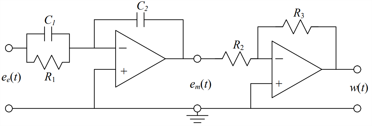
To make the concept of PI control, for example, more concrete, Figure \(\PageIndex{2}\) depicts a specific analog electrical circuit that, in principle, acts as an ideal PI controller. (In practice, a great deal of electronic refinement and conditioning is required to produce a circuit that behaves even close to ideally.) By applying the methods of circuit analysis described in Chapter 5 (homework Problem 5.11), we can show that the PI (\(b_{i}=1\) and \(b_{d}=0\)) constants in Equations \(\ref{eqn:15.1}\) and \(\ref{eqn:15.2}\), expressed in terms of the circuit parameters of Figure \(\PageIndex{2}\), are:

\[P=\frac{R_{3} C_{1}}{R_{2} C_{2}}, \quad \tau_{i}=R_{1} C_{1}\label{eqn:15.3} \]

The detailed design of PID controllers involves a great deal of engineering art as well as engineering science, and it has been developed extensively; see, e.g., Ogata, 2001, Chapter 10. The present chapter is just an introduction to PID control, so we will not delve deeply into design details; instead, we shall explore some of the more general characteristics of P, PI, and PD types of control in the context of relatively simple examples.