The subject of this problem is frequency response of an \(RC\) band-pass filter circuit. The appropriate transfer function is Equation 13.1.5:\[T F_{B}(s)=\frac{L\left[e_{o}\right]}{L\left[e_{i}\right]}=\frac{\tau_{H} s}{\left(\tau_{H} s+1\right)\left(\tau_{L} s+1\right)}=\frac{\omega_{L} s}{\left(s+\omega_{H}\right)\left(s+\omega_{L}\right)} \nonumber \]in which \(\omega_{L} \equiv 1 / \tau_{L}\) is the low-pass break frequency and \(\omega_{H} \equiv 1 / \tau_{H}\) is the high-pass break frequency, and for band-pass functioning it is usually specified that \(\omega_{H}<<\omega_{L}\).
This transfer function has (in the \(s\)-plane) a zero at the origin and poles at \(-\omega_{H}\) and \(-\omega_{L}\). Consider the case for frequency response: \(s=j \omega\), \(\omega \geq 0\). Sketch a graph of the \(s\)-plane that shows the zero and the poles, and sketch on the graph three complex vectors with tails at the zero and the poles, and heads at an arbitrary point \(s=j \omega\) on the positive imaginary axis. Use this graphical construction to derive the frequency-response function in the polar form \(F R F(\omega)=M R(\omega) e^{j \phi(\omega)}\), in which you derive explicit formulas for magnitude ratio \(M R(\omega)\) and phase angle \(\phi(\omega)\). [NOTE: This graphical method of deriving (or calculating) a frequency-response function is somewhat similar to (but simpler than) Evans’ general root-locus method described in Section 16.5, with the “locus” in this case being the positive imaginary axis—see, in particular, the unnumbered figure that directly follows Equation 16.5.7.] Partial answer: \(\phi(\omega)=\pi / 2-\tan ^{-1}\left(\omega / \omega_{H}\right)-\tan ^{-1}\left(\omega / \omega_{L}\right)\) radians
Let \(\omega_{H}=5\) rad/s and \(\omega_{L}=500\) rad/s. Adapt the MATLAB code that produced Figure 17.1.3 to calculate and print a modified Bode diagram for this particular band-pass filter. Your diagram should show that signals at frequencies between about 10 and 200 rad/s are passed through this filter with very little amplitude reduction and relatively little phase change, but that signals at frequencies below about 0.5 rad/s and above about 5,000 rad/s are effectively “filtered out”, removed.
In these exercises, you will use MATLAB function M-files and the MATLAB command fzero to calculate some results that are stated but not explicitly derived in Chapter 17.
Calculate for at least one of the gains \(\Lambda=4,000\) s-2 and \(400,000\) s-2 the more precise value of PM that is annotated on Figure 17.1.3. The procedure is based on the definition of \(\operatorname{PM}(\Lambda)\) in Equation 17.1.10, which shows that you need to find the frequency \(\omega_{\mathrm{PM}}\) at which \(|O L F R F(\omega)|_{\Lambda} \mid=1\), i.e., the gain-crossover frequency. Accordingly, write a function M-file that uses Equation 17.1.7 to compute the quantity \(|O L F R F(\omega)|_{\Lambda} \mid-1\). Then calculate \(\omega_{\mathrm{PM}}\) by calling that function M-file with the fzero command, in which you also include an estimate for \(\omega_{\mathrm{PM}}\) that you read from Figure 17.1.3. Finally, use Equation 17.1.7 again to calculate \(\left.\angle O L F R F(\omega)\right|_{\Lambda}\) for \(\omega=\omega_{\mathrm{PM}}\), and substitute that result into Equation 17.1.10 to obtain the more precise value of \(\operatorname{PM}(\Lambda)\).
Calculate for at least one of the neutral-stability points on Figure 17.4.3 the more precise value of gain (\(\Lambda_{n s 1}\) and/or \(\Lambda_{n s 2}\)) that is stated in the text of Section 17.4. The procedure is based on setting to zero the real part of the appropriate root of the characteristic equation, Equation 17.4.4. Accordingly, write a function M-file that first determines with the root command the three roots of Equation 17.4.4, then uses MATLAB flow control features (perhaps a for loop containing an if loop, or some alternative of your choice) to select the one root of the three that has a positive imaginary part, and finally computes the real part of this root. Then calculate the required \(\Lambda_{n s}\) by calling that function M-file with the fzero command, in which you also include an estimate for the \(\Lambda_{n s}\), which you read from Figure 17.4.3. [See homework Problem 16.8.2 for a different method of solution.]
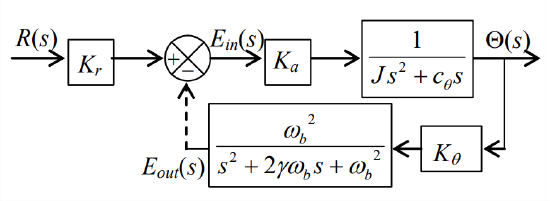
In this problem, re-visit the system of homework Problem 16.5: it is a damped rotor with position feedback that is 2nd order low-pass-filtered. Use the same component values: \(\omega_{b}=300\) rad/s, \(c_{\theta} / J=100\) s-1, and \(\gamma= 1 / \sqrt{2}\). Also as before, denote the varying control-system gain parameter as \(\Lambda \equiv K_{a} K_{\theta} / J\).
Figure \(\PageIndex{1}\) (Copyright; author via source)
Show that the open-loop transfer function is \[O L T F(s) \equiv \frac{E_{o u t}(s)}{E_{i n}(s)}=\Lambda \frac{\omega_{b}^{2}}{s\left(s+c_{\theta} / J\right)\left(s^{2}+2 \gamma \omega_{b} s+\omega_{b}^{2}\right)} \nonumber \]
Homework Problem 16.5.2 showed the following by loci-of-roots analysis for the closed-loop system: Your task is to evaluate stability again for \(\Lambda=3,400\) s-2 and for \(\Lambda=\Lambda_{n s}\), but now using frequency-response criteria. Define the excitation-frequency range of interest to be the band \(10 \leq \omega \leq 1000\) rad/s. First, use appropriate MATLAB commands to calculate the baseline open-loop frequency-response function, i.e., \(\operatorname{OLFRF}(\omega)\) for \(\Lambda=1\) s-2. Now, use MATLAB to calculate and plot on some type (your choice) of Bode diagram the curves of magnitude ratio and phase angle over the defined frequency band, for both \(\Lambda=3,400\) s-2 and \(\Lambda=\Lambda_{n s}\). Estimate from your Bode diagram the gain margin GM (in both decimal form and dB) and the phase margin PM (in degrees) for both values of \(\Lambda\).
\(\Lambda \equiv \Lambda_{n s}=22,000\) s-2 is the neutral-stability gain, the upper limit of stability; and
for \(\Lambda=3,400\) s-2, the system is stable, with the dominant mode being oscillatory and having damping ratio \(\zeta \approx 1 / \sqrt{2}\).
Use MATLAB’s margin function to validate the correctness of your estimated stability margins in part 17.3.2.
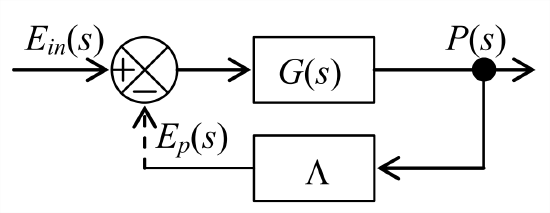
Suppose that you have an LTI rotary motor with unknown transfer function \(G(s)\). The input is a voltage signal \(e_{i n}(t)\), and the output is shaft speed \(\dot{\theta}(t) \equiv p(t)\). You want to control the shaft speed by sensing it with a tachometer, which has variable gain \(\Lambda\), and feeding the tachometer voltage signal \(e_{p}(t)\) back to the input in the standard form shown on the Laplace block diagram.
Figure \(\PageIndex{2}\) (Copyright; author via source)
In order to evaluate the stability of the closed-loop system, you conduct a stepped-sine-sweep frequency-response test on the stable open-loop system, which consists of the motor and the tachometer in series, with the gain set at \(\Lambda=0.4\) volt per rad/s. Specifically, you drive the open-loop system with sinusoidal input voltage \(e_{i n}(t)=V_{i n} \sin \omega t\) with the frequency increasing in small increments through the range \(0.5 \leq \omega \leq 50\) rad/s, you measure at each sine-dwell frequency the steady-state sinusoidal output voltage \(e_{p}(t)=V_{p}(\omega) \sin [\omega t+\phi(\omega)]\), and then you plot the results for \(V_{p}(\omega) / V_{i n}\) and \phi(\omega), leading to the following diagram:
Figure \(\PageIndex{3}\) (Copyright; author via source)
Would the closed-loop system be stable with the tachometer gain for which the above data apply, \(\Lambda=0.4\) volt/(rad/s)? If so, calculate from the diagram above, with as much accuracy as the plots permit, the phase margin PM and gain margin GM of stability. Indicate the graphical representations of your PM and GM on a sketch or photocopy of the diagram.
Would the closed-loop system be driven unstable by any positive values of tachometer gain, \(\Lambda>0\)? If so, estimate those values. Explain your reasoning clearly.
Figure 17.2.1 is in the traditional two-dimensional format of a Nyquist plot, i.e., \(\operatorname{Im}[F R F(\omega)]\) versus \(\operatorname{Re}[F R F(\omega)]\), on which excitation frequency \(\omega\) is the implicit independent variable. But this format might be considered unsatisfactory for many purposes because it lacks a graduated scale for \(\omega\). An enhanced-format Nyquist plot, a three-dimensional plot, can show such a graduated scale of frequency in addition to the scales of the rectangular components, \(\operatorname{Re}[F R F(\omega)]\) and \(\operatorname{Im}[F R F(\omega)]\). In order to explore that format, run in MATLAB the following alternative version of the commands that produced Figure 17.2.1, which applies, in particular, the plot3 command to plot three-dimensionally:
>> wn=2*pi;zt=0.2;
>> w=wn*(0:0.05:2.5);
>> frf=wn^2./(wn^2-w.^2+j*2*zt*wn*w);
>> plot3(real(frf),imag(frf),w/wn),grid
>> axis equal
These commands should produce a three-dimensional plot on which the \(\operatorname{Re}[F R F(\omega)]\) axis (the \(x\)-axis) extends from \(\approx-1\) to \(\approx+1.5\), the \(\operatorname{Im}[F R F(\omega)]\) axis (the \(y\)-axis) extends from 0 to −2.5, and the \(\omega / \omega_{n}\) axis (the \(z\)-axis) extends from 0 to 2.5. Make a print of the initial plot, which probably will be from the “Default 3-D View” (azimuth = \(-37.5^{\circ}\), elevation = \(-30^{\circ}\); Orthographic, not Perspective). The Reference 3-D View, azimuth = \(0^{\circ}\) and elevation = \(0^{\circ}\), is from \(y=-\infty\) looking in exactly the \(+ y\) direction, so it is a two-dimensional projection of the \(x\)-\(z\) plane. Azimuth angle is positive rotation (in the sense of the right-hand rule) of the viewpoint about the \(z\) axis, relative to the Reference 3-D View; thus, for example, the view azimuth = \(90^{\circ}\) and elevation = \(0^{\circ}\) is from \(x=+\infty\) looking in exactly the \(− x\) direction, a two-dimensional projection of the \(y\)-\(z\) plane.
Consider two consecutive excitation frequencies in a frequency-response experiment, denoted as \(\omega_{i}\) and \(\omega_{j}\), with \(\omega_{j}>\omega_{i}\) [e.g., two consecutive values in the series represented by the MATLAB command w=wn*(0:0.05:2.5)], and denote \(\Delta \omega_{i j}=\omega_{j}-\omega_{i}\); denote the change from \(\omega_{i}\) and \(\omega_{j}\) of the in-phase component \(\operatorname{Re}[F R F(\omega)]\) as \(\Delta x_{i j}\), and that of the quadrature component \(\operatorname{Im}[F R F(\omega)]\) as \(\Delta y_{i j}\); then the line segment between those two points in the \(\operatorname{Im}[F R F(\omega)]\)-versus-\(\operatorname{Re}[F R F(\omega)]\) plane (e.g., Figure 17.2.1, the \(x\)-\(y\) plane) is \(\Delta s_{i j} =\sqrt{\Delta x_{i j}^{2}+\Delta y_{i j}^{2}}\). Engineers who conduct stepped-sine-sweep frequency-response vibration tests on resonant systems (such as that of this problem) consider the rate of change \(\Delta s_{i j} / \Delta \omega_{i j}\) to be a physically significant quantity that leads to experimental determination of a system’s natural frequency, \(\omega_{n}\). Describe how your three-dimensional Nyquist plots (from whatever viewpoints are required) demonstrate that \(\Delta s_{i j} / \Delta \omega_{i j}\) is maximum at excitation frequencies near \(\omega_{n}\), but is below the maximum at frequencies both above and below \(\omega_{n}\).
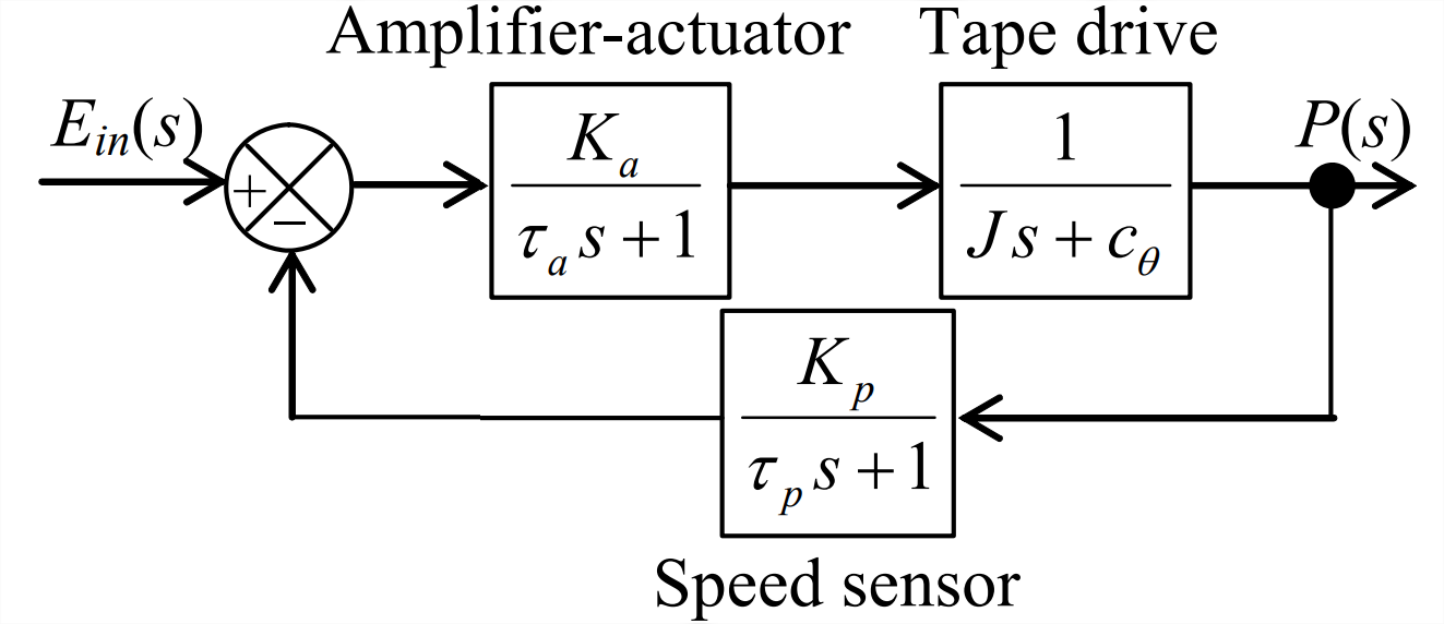
In this problem, re-visit the system of homework Problem 16.7: the Laplace block diagram of the speed-control system of a magnetic-tape drive is shown in the figure on the next page. The operator setting is input voltage signal \(e_{i n}(t)\), the Laplace transform of which is \(E_{i n}(s)\). Each major sub-system of the control system functions as a 1st order system. The sub-system consisting of a power amplifier and a torque actuator has variable sensitivity \(K_{a}\) (N-m/V) and time constant \(\tau_{a}=1.0\) s. The tape drive has rotational inertia \(J=4.0\) N-m per rad/s2 and lubricated-shaft viscous damping constant \(c_{\theta}=1.0\) N-m per rad/s; the output of the tape drive in this application is rotational speed \(p(t)\) in rad/s [with Laplace transform \(P(s)\)], not rotational position \(\theta(t)\). The rotational-speed sensor in the feedback branch has sensitivity \(K_p = 1.250\) V per rad/s; this sensor is sufficiently slow relative to the other sub-systems that we must account for its time constant, \(\tau_{p}=0.50\) s.
Figure \(\PageIndex{4}\) (Copyright; author via source)
Defining the control gain parameter as \(\Lambda=K_{a} K_{p} /\left(J \tau_{a} \tau_{p}\right)\), with units of s-3, show that the closed-loop transfer function is \(\frac{P(s)}{E_{i n}(s)}=\frac{K_{a}}{J \tau_{a}} \frac{s+\tau_{p}^{-1}}{\left(s+c_{\theta} / J\right)\left(s+\tau_{a}^{-1}\right)\left(s+\tau_{p}^{-1}\right)+\Lambda}\). Consider response to a unit-step input, \(e_{i n}(t)=(1.0 \mathrm{V}) H(t)\). Use the final-value theorem (assuming system stability) to find an equation in terms of the system parameters for the steady-state response, after all transients have decayed, \(\lim _{t \rightarrow \infty} p(t)\). Select the value of sensitivity \(K_a\) that makes the overall steady-state sensitivity of the control system be 0.750 rad/s per volt, then calculate gain \(\Lambda\) corresponding to that value of \(K_a\). (partial solution: \(\Lambda=7.50\) s-3)
Show that the open-loop frequency-response function can be written as \(O \operatorname{LFRF}(\omega)= \Lambda \times \frac{1}{\left(j \omega+c_{\theta} / J\right)\left(j \omega+\tau_{a}^{-1}\right)\left(j \omega+\tau_{p}^{-1}\right)}\). Calculate for the given parameter values the phase-crossover frequency \(\omega_{n s}\), i.e., the frequency at which \(\angle O L F R F(\omega)=-\pi\) radians \(= -180^{\circ}\); this task will require the numerical solution of a transcendental equation, which you might want to accomplish by applying the MATLAB function fzero in the manner described in homework Problem 17.2. Next, calculate for the baseline case, \(\Lambda=1\) s-3, the magnitude ratio at phase crossover, \(M R_{1}\left(\omega_{n s}\right)\), and the corresponding gain margin, GM1. (partial solution: GM1 = 8.4375)
Now consider the gain determined in part (a), \(\Lambda=7.50\) s-3. Calculate the magnitude ratio at phase crossover, \(M R_{7.50}\left(\omega_{n s}\right)\), and the corresponding gain margin, \(\mathrm{GM}_{7.50}\). Calculate the phase margin, \(\mathrm{PM}_{7.50}\), using the equation for \(O L F R F(\omega)\) of part (b)—to do this, you will need first to find the gain-crossover frequency \(\omega_{1}\) [\(M R_{7.50}\left(\omega_{1}\right)=1\)], which you might want to accomplish by applying again the MATLAB function fzero in the manner described in homework Problem 17.2; then you will need to calculate phase angle \(\angle O L F R F\left(\omega_{1}\right)\) to use in the definition of phase margin.
To validate your work in the previous parts, produce a diagram showing the Nyquist plots for both values of gain, \(\Lambda=1\) and 7.50 s-3; you might wish just to adapt for this case the MATLAB code that produced Figure 17.4.4. What is your assessment, based on the gain and phase margins, of the control system with gain \(\Lambda=7.50\) s-3?
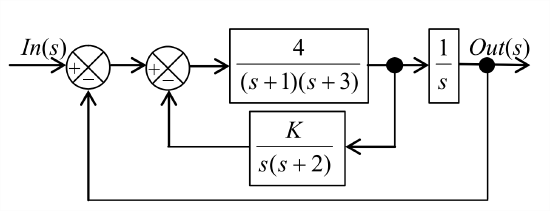
Consider the feedback control system depicted in the Laplace block diagram at right. Assume that units of all constants are consistent, and do not bother to label units.
Figure \(\PageIndex{5}\) (Copyright; author via source)
Combine the two feedback loops with block-diagram algebra to show that the forward-branch and feedback-branch transfer functions can be written, respectively, as: \(G(s)=\frac{4}{s(s+1)(s+3)}\) and \(H(s)=\frac{s+(2+K)}{s+2}\). Apply Routh’s criteria, as described in homework Problem 16.9.3, to determine the range of the sensitivity constant \(K\) over which the control system is stable.
Use any method of your choosing to determine the value of \(K\) for which the phase margin PM is approximately \(35^{\circ}\). Note that the characteristic equation of this system does not have the form of either of Equations 16.6.3: this \(K\) does not play the role of \(\Lambda\) in Equations 16.6.3. Therefore, many of the equations developed in Chapter 17, such as Equations 17.1.11-17.1.16, are not applicable in this problem.
To validate your work in parts (a) and (b), produce a diagram showing the Nyquist plots for two values of \(K\): both that for neutral stability (the upper-bound \(K\) for system stability), and that for \(\mathrm{PM} \approx 35^{\circ}\); you might wish just to adapt for this case the MATLAB code that produced Figure 17.4.4. Explain the features of the Nyquist plots that confirm the correctness of your results in parts (a) and (b), using annotations on the diagram and/or written discussion.
Your task in this problem is to derive, with the assistance of MATLAB’s symbolic capabilities, the “steady-state” response Equation 17.3.2, which includes the unstable linear drift due to the open-loop transfer function’s pole at \(s=0+j 0\). Because the equations that MATLAB produces are long and complicated, it will be advantageous to separate the voltage input function Equation 17.3.1 into the following two parts:\[e_{i n_{1}}(t)=E_{i n} \sin \omega t \quad \text { and } \quad e_{i n 2}(t)=E_{o f f} H(t) \nonumber \]For each of these parts individually you will seek the voltage output solution, respectively, \(e_{\text {outl}}(t)\) and \(e_{\text {out} 2}(t)\), then you will add the two to obtain the total response.
The Laplace transform of \(e_{\text {outl}}(t)\), with the use of Equation 17.1.2 and Equation 2.4.7, is\[L\left[e_{\text {out } 1}(t)\right]=L\left[e_{i n 1}(t)\right] \times O L T F(s)=E_{\text {in}} \frac{\omega}{s^{2}+\omega^{2}} \times \Lambda \frac{\omega_{b}}{s\left(s+c_{\theta} / J\right)\left(s+\omega_{b}\right)} \nonumber \]You might be able to find the inverse transform of this equation in some reference, but it is likely that a more efficient process is to define the equation symbolically in MATLAB and then to use the ilaplace command to find the inverse transform. The less appealing aspect of this approach is that MATLAB’s initial solution will probably be long and difficult to interpret. To convert the initial solution equation into a more transparent form, use the simple and pretty commands. You seek the “steady-state” response, so discard (from the equation displayed after use of pretty) the transient terms involving the time functions \(e^{-\left(c_{\theta} / J\right) t}\) and \(e^{-\omega_{b} t}\). At this point, you should be able to express the solution in the form:\[\frac{e_{o u t 1}(t)}{E_{i n}}=\frac{\Lambda}{\omega\left(c_{\theta} / J\right)}+\Lambda \omega_{b} \frac{-\left(c_{\theta} / J+\omega_{b}\right) \sin \omega t+\left[\omega-\left(c_{\theta} / J\right) \omega_{b} / \omega\right] \cos \omega t}{\left[\omega^{2}+\left(c_{\theta} / J\right)^{2}\right]\left(\omega^{2}+\omega_{b}^{2}\right)} \nonumber \]The second right-hand-side term above is clearly a frequency-response term; but it is not yet expressed in the form from which equations for magnitude ratio and phase angle can be written, so you need to convert it into that form. Use the general trigonometric identity \(\sin \theta \times \cos \phi+\cos \theta \times \sin \phi=\sin (\theta+\phi)\), and follow the procedure described in Equations 4.3.2-4.3.5, to show that \(C \sin \omega t+S \cos \omega t=\sqrt{C^{2}+S^{2}} \sin (\omega t+\phi)\), where \(\phi = \tan ^{-1}(S / C)\). Use this result to write explicit equations, in terms of \(c_{\theta} / J\) and \(\omega_b\) and \(\omega\), for magnitude ratio \(M R(\omega)\) and phase angle \(\phi(\omega)\). In the remainder of this problem, do not write out again those somewhat lengthy equations; instead, just use the symbols \(M R(\omega)\) and \(\phi(\omega)\).
Use Equation 17.1.2 again and MATLAB’s ilaplace command in order to solve for output voltage \(e_{\text {out } 2}(t)\) in response to \(e_{i n 2}(t)=E_{o f f} H(t)\).
Combine the response equations of parts (a) and (b) to write the complete solution \(e_{\text {out}}(t)=e_{\text {out} 1}(t)+e_{\text {out} 2}(t)\), the “steady-state” response Equation 17.3.2:\[e_{o u t}(t)=E_{i n}\left(M R(\omega) \times \sin (\omega t+\phi(\omega))+\frac{\Lambda}{\omega\left(c_{\theta} / J\right)}\right)+E_{o f f} \frac{\Lambda J}{c_{\theta}}\left[t-\frac{\left(c_{\theta} / J+\omega_{b}\right)}{\left(c_{\theta} / J\right) \omega_{b}}\right] \nonumber \]