17.4: The Nyquist Stability Criterion

Section 17.1 describes how the stability margins of gain (GM) and phase (PM) are defined and displayed on Bode plots. It is informative and it will turn out to be even more general to extract the same stability margins from Nyquist plots of frequency response. To begin this study, we will repeat the Nyquist plot of Figure 17.2.2, the closed-loop neutral-stability case, for which \(\Lambda=\Lambda_{n s}=40,000\) s^-2 and \(\omega_{n s}=100 \sqrt{3}\) rad/s, but over a narrower band of excitation frequencies, \(100 \leq \omega \leq 1,000\) rad/s, or \(1 / \sqrt{3} \leq \omega / \omega_{n s} \leq 10 / \sqrt{3}\); the intent here is to restrict our attention primarily to frequency response for which the phase lag exceeds about 150°, i.e., for which the frequency-response curve in the \(OLFRF\)-plane is somewhat close to the negative real axis. Moreover, we will add to the same graph the Nyquist plots of frequency response for a case of positive closed-loop stability with \(\Lambda=1 / 2 \Lambda_{n s}=20,000\) s^-2, and for a case of closed-loop instability with \(\Lambda= 2 \Lambda_{n s}=80,000\) s^-2. The MATLAB commands follow that calculate [from Equations 17.1.7 and 17.1.12] and plot these cases of open-loop frequency-response function, and the resulting Nyquist diagram (after additional editing):

>> wb=300;coj=100;w=logspace(2,3,200);

>> olfrf01=wb./(j*w.*(j*w+coj).*(j*w+wb));

>> olfrf20k=20e3*olfrf01;olfrf40k=40e3*olfrf01;olfrf80k=80e3*olfrf01;

>> plot(real(olfrf80k),imag(olfrf80k),real(olfrf40k),imag(olfrf40k),…

real(olfrf20k),imag(olfrf20k)),grid

Figure \(\PageIndex{1}\): Nyquist plots of Equation 17.1.7, open-loop frequency-response functions (\(OLFRF\)) for \(\Lambda=(1 / 2,1, \text { and } 2) \times \Lambda_{n s}\) for the system in Figure 17.1.2, with parameters \(\omega_b = 300\) s^-1, \(c_{\theta} / J=100\) s^-1, and \(\omega_{n s}=\sqrt{ \omega_{b} \times c_{\theta} / J}=173.2\) rad/s. (Copyright; author via source)

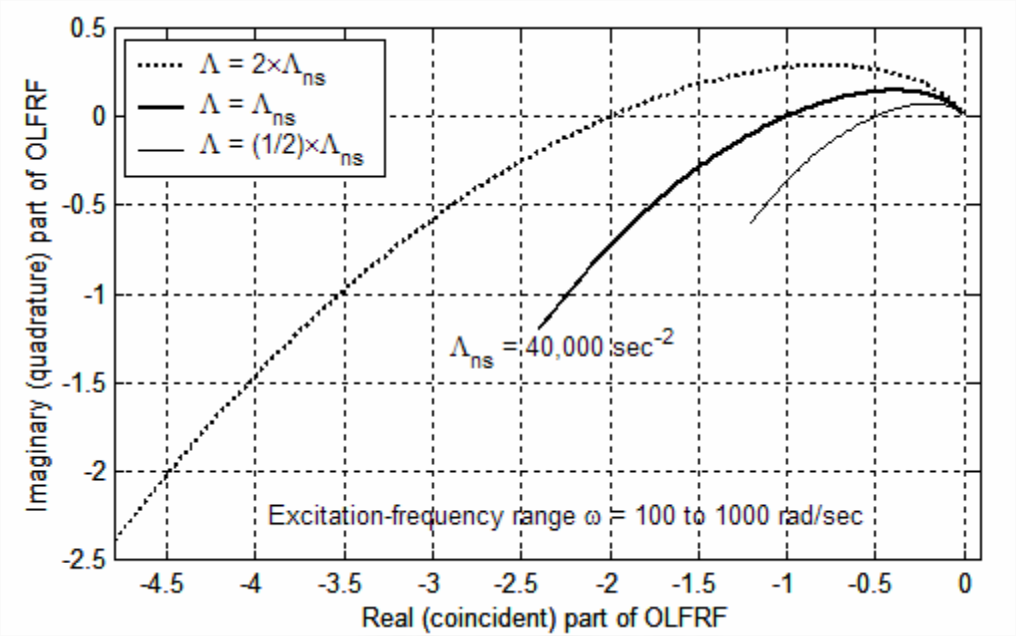
Gain margin and phase margin are present and measurable on Nyquist plots such as those of Figure \(\PageIndex{1}\). Gain margin (GM) is defined by Equation 17.1.8, from which we find

\[\frac{1}{G M(\Lambda)}=|O L F R F(\omega)|_{\mid} \mid \text {at }\left.\angle O L F R F(\omega)\right|_{\Lambda}=-180^{\circ}\label{eqn:17.17} \]

Equation \(\ref{eqn:17.17}\) is illustrated on Figure \(\PageIndex{2}\) for both closed-loop stable and unstable cases. Note that a closed-loop-stable case has \(0<1 / \mathrm{GM}_{\mathrm{S}}<1\) so that \(\mathrm{GM}_{\mathrm{S}}>1\), and a closed-loop-unstable case has \(1 / \mathrm{GM}_{\mathrm{U}}>1\) so that \(0<\mathrm{GM}_{\mathrm{U}}<1\).

Figure \(\PageIndex{2}\): Schematic Nyquist plots of open-loop frequency-response functions (\(OLFRF\)) for closed-loop-stable and –unstable cases. (Copyright; author via source)

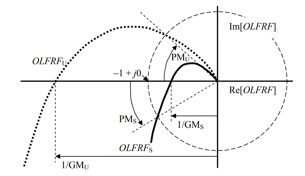
We can measure phase margin directly by drawing on the Nyquist diagram a circle with radius of 1 unit and centered on the origin of the complex \(OLFRF\)-plane, so that it passes through the important point \(-1+j 0\). Phase margin is defined by

\[\operatorname{PM}(\Lambda)=180^{\circ}+\left(\left.\angle O L F R F(\omega)\right|_{\Lambda} \text { at }|O L F R F(\omega)|_{\Lambda} \mid=1\right)\label{eqn:17.7} \]

Phase margins are indicated graphically on Figure \(\PageIndex{2}\). The positive \(\mathrm{PM}_{\mathrm{S}}\) for a closed-loop-stable case is the counterclockwise angle from the negative \(\operatorname{Re}[O L F R F]\) axis to the intersection of the unit circle with the \(OLFRF_S\) curve; conversely, the negative \(\mathrm{PM}_U\) for a closed-loop-unstable case is the clockwise angle from the negative \(\operatorname{Re}[O L F R F]\) axis to the intersection of the unit circle with the \(OLFRF_U\) curve.

Note on Figure \(\PageIndex{2}\) that the phase-crossover point (phase angle \(\phi=-180^{\circ}\)) and the gain-crossover point (magnitude ratio \(MR = 1\)) of an \(FRF\) are clearly evident on a Nyquist plot, perhaps even more naturally than on a Bode diagram. On the other hand, a Bode diagram displays the phase-crossover and gain-crossover frequencies, which are not explicit on a traditional Nyquist plot.

With a little imagination, we infer from the Nyquist plots of Figure \(\PageIndex{1}\) that the open-loop system represented in that figure has \(\mathrm{GM}>0\) and \(\mathrm{PM}>0\) for \(0<\Lambda<\Lambda_{\mathrm{ns}}\), and that \(\mathrm{GM}>0\) and \(\mathrm{PM}>0\) for all values of gain \(\Lambda\) greater than \(\Lambda_{\mathrm{ns}}\); accordingly, the associated closed-loop system is stable for \(0<\Lambda<\Lambda_{\mathrm{ns}}\), and unstable for all values of gain \(\Lambda\) greater than \(\Lambda_{\mathrm{ns}}\). Thus, this physical system (of Figures 16.3.1, 16.3.2, and 17.1.2) is considered a “common” system, for which gain margin and phase margin provide clear and unambiguous metrics of stability. Let us consider next an “uncommon” system, for which the determination of stability or instability requires a more detailed examination of the stability margins. Suppose that the open-loop transfer function of a system is¹

\[G(s) \times H(s) \equiv O L T F(s)=\Lambda \frac{s^{2}+4 s+104}{(s+1)\left(s^{2}+2 s+26\right)}=\Lambda \frac{s^{2}+4 s+104}{s^{3}+3 s^{2}+28 s+26}\label{eqn:17.18} \]

You should be able to show that the zeros of this transfer function in the complex \(s\)-plane are at (\(−2 ± j10\)), and the poles are at (\(−1 + j0\)) and (\(−1 ± j5\)).

In order to establish the reference for stability and instability of the closed-loop system corresponding to Equation \(\ref{eqn:17.18}\), we determine the loci of roots from the characteristic equation, \(1+G H=0\), or

\[s^{3}+3 s^{2}+28 s+26+\Lambda\left(s^{2}+4 s+104\right)=s^{3}+(3+\Lambda) s^{2}+4(7+\Lambda) s+26(1+4 \Lambda)=0\label{17.19} \]

The following MATLAB commands, adapted from the code that produced Figure 16.5.1, calculate and plot the loci of roots:

Lm=[0 .2 .4 .7 1 1.5 2.5 3.7 4.75 6.5 9 12.5 15 18.5 25 35 50 70 125 250];

Np=length(Lm);

for i=1:Np;

a2=3+Lm(i);a3=4*(7+Lm(i));a4=26*(1+4*Lm(i));

p(i,1:3)=roots([1 a2 a3 a4]).';

end

plot(p,'kx'),grid,xlabel('Real part of pole (sec^-^1)')

ylabel('Imaginary part of pole (sec^-^1)')

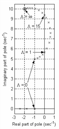
The significant roots of Equation \(\ref{eqn:17.19}\) are shown on Figure \(\PageIndex{3}\): the complete locus of oscillatory roots with positive imaginary parts is shown; only the beginning of the locus of real (exponentially stable) roots is shown, since those roots become progressively more negative as gain \(\Lambda\) increases from the initial small values. The oscillatory roots on Figure \(\PageIndex{3}\) show that the closed-loop system is stable for \(\Lambda=0\) up to \(\Lambda \approx 1\), it is unstable for \(\Lambda \approx 1\) up to \(\Lambda \approx 15\), and it becomes stable again for \(\Lambda\) greater than \(\approx 15\). We regard this closed-loop system as being “uncommon” or unusual because it is stable for small and large values of gain \(\Lambda\), but unstable for a range of intermediate values.

If we were to test experimentally the open-loop part of this system in order to determine the stability of the closed-loop system, what would the open-loop frequency responses be for different values of gain \(\Lambda\)? To simulate that testing, we have from Equation \(\ref{eqn:17.18}\), the following equation for the frequency-response function:

\[O L F R F(\omega) \equiv O L T F(j \omega)=\Lambda \frac{104-\omega^{2}+4 \times j \omega}{(1+j \omega)\left(26-\omega^{2}+2 \times j \omega\right)}\label{eqn:17.20} \]

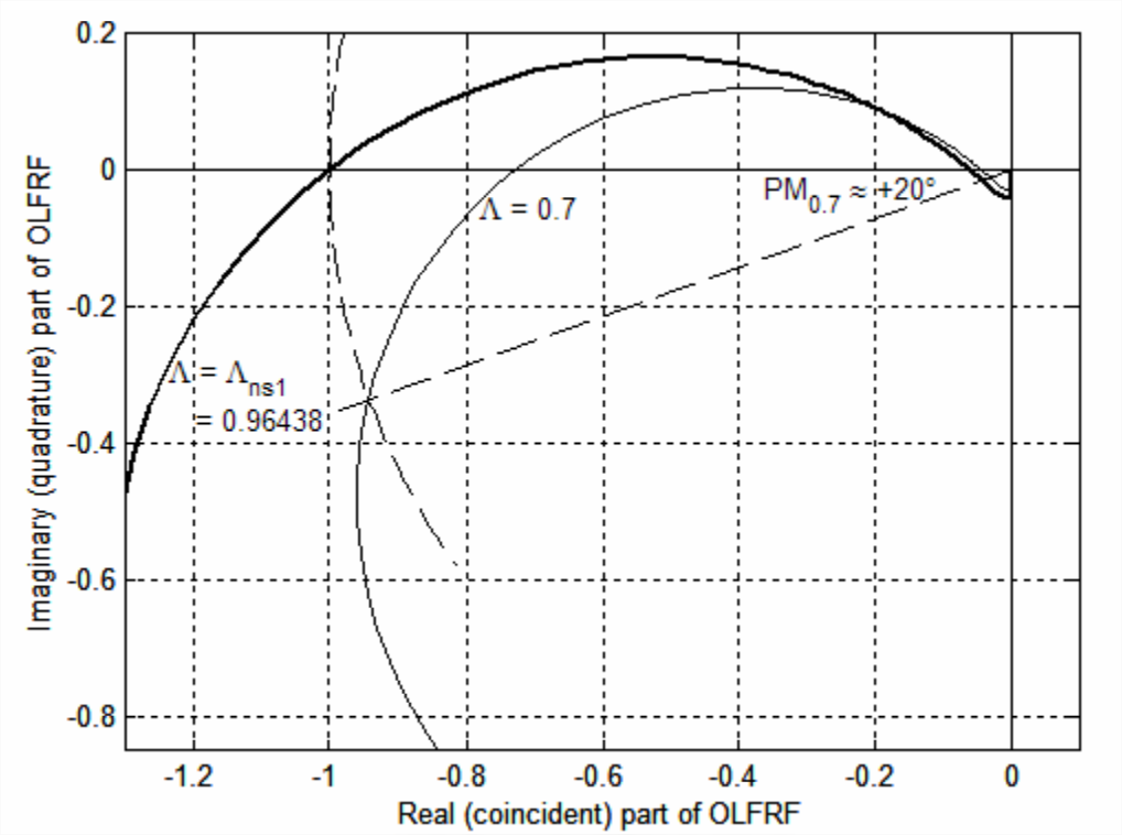
Let us begin this study by computing \(\operatorname{OLFRF}(\omega)\) and displaying it on Nyquist plots for a low value of gain, \(\Lambda=0.7\) (for which the closed-loop system is stable), and for the value corresponding to the transition from stability to instability on Figure \(\PageIndex{3}\), which we denote as \(\Lambda_{n s 1} \approx 1\). The value of \(\Lambda_{n s 1}\) is not exactly 1, as Figure \(\PageIndex{3}\) might suggest; see homework Problem 17.2(b) for calculation of the more precise value \(\Lambda_{n s 1}=0.96438\). The following MATLAB commands calculate and plot the two frequency responses and also, for determining phase margins as shown on Figure \(\PageIndex{2}\), an arc of the unit circle centered on the origin of the complex \(O L F R F(\omega)\)-plane.

Figure \(\PageIndex{3}\): Loci of roots of Equation \(\ref{eqn:17.19}\). (Copyright; author via source)

>> w=3.4*logspace(0,2,500);

>> olfrf01=(104-w.^2+4*j*w)./((1+j*w).*(26- w.^2+2*j*w));

>> olfrf007=0.7*olfrf01;

>> plot(real(olfrf007),imag(olfrf007)),grid

>> cirangrad=0.8*pi:0.01:1.2*pi;

>> hold,plot(cos(cirangrad),sin(cirangrad))

Current plot held

>> olfrfns1=0.96438*olfrf01;

>> plot(real(olfrfns1),imag(olfrfns1))

The portions of both Nyquist plots (for \(\Lambda=0.7\) and \(\Lambda=\Lambda_{n s 1}\)) that are closest to the negative \(\operatorname{Re}[O L F R F]\) axis are shown on Figure \(\PageIndex{4}\) (next page). Observe on Figure \(\PageIndex{4}\) the small loops beneath the negative \(\operatorname{Re}[O L F R F]\) axis as driving frequency becomes very high: the frequency responses approach zero from below the origin of the complex \(OLFRF\)-plane. This is distinctly different from the Nyquist plots of a more “common” open-loop system on Figure \(\PageIndex{1}\), which approach the origin from above as frequency becomes very high. Another aspect of the difference between the plots on the two figures is particularly significant: whereas the plots on Figure \(\PageIndex{1}\) cross the negative \(\operatorname{Re}[O L F R F]\) axis only once as driving frequency \(\omega\) increases, those on Figure \(\PageIndex{4}\) have two phase crossovers, i.e., the phase angle is −180° for two different values of \(\omega\). Since on Figure \(\PageIndex{4}\) there are two different frequencies at which \(\left.\angle O L F R F(\omega)\right|_{\Lambda}=-180^{\circ}\), the definition of gain margin in Equations 17.1.8 and \(\ref{eqn:17.17}\) is ambiguous: at which, if either, of the phase crossovers is it appropriate to read the quantity \(1 / \mathrm{GM}\), as shown on \(\PageIndex{2}\)? Which, if either, of the values calculated from that reading, \(\mathrm{GM}=(1 / \mathrm{GM})^{-1}\) is a legitimate metric of closed-loop stability? \(\PageIndex{4}\) includes the Nyquist plots for both \(\Lambda=0.7\) and \(\Lambda =\Lambda_{n s 1}\), the latter of which by definition crosses the negative \(\operatorname{Re}[O L F R F]\) axis at the point \(-1+j 0\), not far to the left of where the \(\Lambda=0.7\) plot crosses at about \(-0.73+j 0\); therefore, it might be that the appropriate value of gain margin for \(\Lambda=0.7\) is found from \(1 / \mathrm{GM}_{0.7} \approx 0.73\), so that \(\mathrm{GM}_{0.7} \approx 1.37=2.7\) dB, a small gain margin indicating that the closed-loop system is just weakly stable. If, on the other hand, we were to calculate gain margin using the other phase crossing, at about \(-0.04+j 0\), then that would lead to the exaggerated \(\mathrm{GM} \approx 25=28\) dB, which is obviously a defective metric of stability. Note that the phase margin for \(\Lambda=0.7\), found as shown on Figure \(\PageIndex{2}\), is quite clear on Figure \(\PageIndex{4}\) and not at all ambiguous like the gain margin: \(\mathrm{PM}_{0.7} \approx+20^{\circ}\); this value also indicates a stable, but weakly so, closed-loop system.

Figure \(\PageIndex{4}\): Nyquist plots, Equation \(\ref{eqn:17.20}\), open-loop frequency-response functions (\(OLFRF\)) for \(\Lambda=0.7\) and \(\Lambda=\Lambda_{n s 1}=0.96438\) in the system of Equation \(\ref{eqn:17.18}\). (Copyright; author via source)

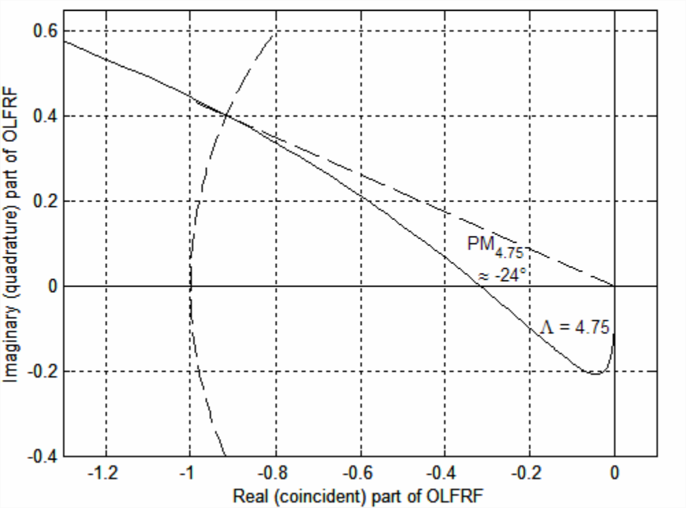
Let us continue this study by computing \(OLFRF(\omega)\) and displaying it as a Nyquist plot for an intermediate value of gain, \(\Lambda=4.75\), for which Figure \(\PageIndex{3}\) shows the closed-loop system is unstable. The following MATLAB commands calculate [from Equations 17.1.12 and \(\ref{eqn:17.20}\)] and plot the frequency response and an arc of the unit circle centered at the origin of the complex \(OLFRF(\omega)\)-plane.

w=3.4*logspace(0,2,500);

olfrf01=(104-w.^2+4*j*w)./((1+j*w).*( 26-w.^2+2*j*w));

>> olfrf0475=4.75*olfrf01;

>> plot(real(olfrf0475),imag(olfrf0475)),grid

>> cirangrad=0.8*pi:0.01:1.2*pi;

>> hold,plot(cos(cirangrad),sin(cirangrad))

The portion of the Nyquist plot for gain \(\Lambda=4.75\) that is closest to the negative \(\operatorname{Re}[O L F R F]\) axis is shown on Figure \(\PageIndex{5}\). The \(\Lambda=\Lambda_{n s 1}\) plot of Figure \(\PageIndex{4}\) is expanded radially outward on Figure \(\PageIndex{5}\) by the factor of \(4.75 / 0.96438=4.9254\), so the loop for high frequencies beneath the negative \(\operatorname{Re}[O L F R F]\) axis is more prominent than on Figure \(\PageIndex{4}\). The frequency-response curve leading into that loop crosses the \(\operatorname{Re}[O L F R F]\) axis at about \(-0.315+j 0\); if we were to use this phase crossover to calculate gain margin, then we would find \(\mathrm{GM} \approx 1 / 0.315=3.175=10.0\) dB. Moreover, if we apply for this system with \(\Lambda=4.75\) the MATLAB margin command to generate a Bode diagram in the same form as Figure 17.1.5, then MATLAB annotates that diagram with the values \(\mathrm{GM}=10.007\) dB and \(\mathrm{PM}=-23.721^{\circ}\) (the same as PM4.75 shown approximately on Figure \(\PageIndex{5}\)). We know from Figure \(\PageIndex{3}\) that this case of \(\Lambda=4.75\) is closed-loop unstable. However, the positive gain margin 10 dB suggests positive stability. The negative phase margin indicates, to the contrary, instability. Clearly, the calculation \(\mathrm{GM} \approx 1 / 0.315\) is a defective metric of stability. The other phase crossover, at \(-4.9254+j 0\) (beyond the range of Figure \(\PageIndex{5}\)), might be the appropriate point for calculation of gain margin, since it at least indicates instability, \(\mathrm{GM}_{4.75}=1 / 4.9254=0.20303=-13.85\) dB.

Figure \(\PageIndex{5}\): Nyquist plot, Equation \(\ref{eqn:17.20}\), open-loop frequency-response function (\(OLFRF\)) for (\Lambda=4.75\) in the system of Equation \(\ref{eqn:17.18}\). (Copyright; author via source)

Let us complete this study by computing \(\operatorname{OLFRF}(\omega)\) and displaying it on Nyquist plots for the value corresponding to the transition from instability back to stability on Figure \(\PageIndex{3}\), which we denote as \(\Lambda_{n s 2} \approx 15\), and for a slightly higher value, \(\Lambda=18.5\), for which the closed-loop system is stable. The value of \(\Lambda_{n s 2}\) is not exactly 15, as Figure \(\PageIndex{3}\) might suggest; see homework Problem 17.2(b) for calculation of the more precise value \(\Lambda_{n s 2} = 15.0356\). The portions of both Nyquist plots (for \(\Lambda_{n s 2}\) and \(\Lambda=18.5\)) that are closest to the negative \(\operatorname{Re}[O L F R F]\) axis are shown on Figure \(\PageIndex{6}\), which was produced by the MATLAB commands that produced Figure \(\PageIndex{4}\), except with gains 18.5 and \(\Lambda_{n s 2}\) replacing, respectively, gains 0.7 and \(\Lambda_{n s 1}\).

Figure \(\PageIndex{6}\): Nyquist plots, Equation \(\ref{eqn:17.20}\), open-loop frequency-response functions (\(OLFRF\)) for \(\Lambda=\Lambda_{n s 2}=15.0356\) and \(\Lambda=18.5\) in the system of Equation \(\ref{eqn:17.18}\). (Copyright; author via source)

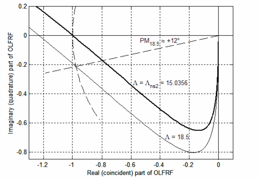
For gain \(\Lambda = 18.5\), there are two phase crossovers: one evident on Figure \(\PageIndex{6}\) at \(-18.5 / 15.0356+j 0=-1.230+j 0\), and the other way beyond the range of Figure \(\PageIndex{6}\) at \(-18.5 / 0.96438+j 0=-19.18+j 0\). We know from Figure \(\PageIndex{3}\) that the closed-loop system with \(\Lambda = 18.5\) is stable, albeit weakly. However, the gain margin calculated from either of the two phase crossovers suggests instability, showing that both are deceptively defective metrics of stability. On the other hand, the phase margin shown on Figure \(\PageIndex{6}\), \(\mathrm{PM}_{18.5} \approx+12^{\circ}\), correctly indicates weak stability.

We draw the following conclusions from the discussions above of Figures \(\PageIndex{3}\) through \(\PageIndex{6}\), relative to an “uncommon” system with an open-loop transfer function such as Equation \(\ref{eqn:17.18}\):

1. gain margin as defined on Figure \(\PageIndex{5}\) can be an ambiguous, unreliable, and even deceptive metric of closed-loop stability;
2. phase margin as defined on Figure \(\PageIndex{5}\), on the other hand, is usually an unambiguous and reliable metric, with \(\mathrm{PM}>0\) indicating closed-loop stability, and \(\mathrm{PM}<0\) indicating closed-loop instability.

Conclusion 2. regarding phase margin is a form of the Nyquist stability criterion, a form that is pertinent to systems such as that of Equation \(\ref{eqn:17.18}\); it is not the most general form of the criterion, but it suffices for the scope of this introductory textbook.

Proofs of the general Nyquist stability criterion are based on the theory of complex functions of a complex variable; many textbooks on control theory present such proofs, one of the clearest being that of Franklin, et al., 1991, pages 261-280. This reference shows that the form of stability criterion described above [Conclusion 2.] is not sufficiently general to handle all cases that might arise. For example, the unusual case of an open-loop system that has unstable poles requires the general Nyquist stability criterion. However, the actual hardware of such an open-loop system could not be subjected to frequency-response experimental testing due to its unstable character, so a control-system engineer would find it necessary to analyze a mathematical model of the system. It is likely that the most reliable theoretical analysis of such a model for closed-loop stability would be by calculation of closed-loop loci of roots, not by calculation of open-loop frequency response. Another unusual case that would require the general Nyquist stability criterion is an open-loop system with more than one gain crossover, i.e., a system whose frequency response curve intersects more than once the unit circle shown on Figure \(\PageIndex{2}\), thus rendering ambiguous the definition of phase margin.

We conclude this chapter on frequency-response stability criteria by observing that margins of gain and phase are used also as engineering design goals. For example, Brogan, 1974, page 25, wrote “Experience has shown that acceptable transient response will usually require stability margins on the order of \(\mathrm{PM}>30^{\circ}\), \(\mathrm{GM}>6\) dB.” Franklin, et al., 1991, page 285, wrote “Many engineers think directly in terms of \(\text { PM }\) in judging whether a control system is adequately stabilized. In using \(\text { PM }\) this way, a phase margin of 30° is often judged to be the lowest acceptable \(\text { PM }\), with values above 30° desirable.”

¹This transfer function was concocted for the purpose of demonstration. It does not represent any specific real physical system, but it has characteristics that are representative of some real systems. Gain \(\Lambda\) has physical units of s^-1, but we will not bother to show units in the following discussion.