
1.8: Continuous Time Complex Exponential
- Page ID
- 23114

Introduction
Complex exponentials are some of the most important functions in our study of signals and systems. Their importance stems from their status as eigenfunctions of linear time invariant systems. Before proceeding, you should be familiar with complex numbers.
The Continuous Time Complex Exponential
Complex Exponentials
The complex exponential function will become a critical part of your study of signals and systems. Its general continuous form is written as
\[Ae^{st} \nonumber \]
where \(s=\sigma+i \omega\) is a complex number in terms of \(\sigma\), the attenuation constant, and \(\omega\) the angular frequency.
Euler's Formula
The mathematician Euler proved an important identity relating complex exponentials to trigonometric functions. Specifically, he discovered the eponymously named identity, Euler's formula, which states that
\[e^{j x}=\cos (x)+j \sin (x) \nonumber \]
which can be proven as follows.
In order to prove Euler's formula, we start by evaluating the Taylor series for \(e^z\) about \(z=0\), which converges for all complex \(z\), at \(z=jx\). The result is
\[\begin{align}
e^{j x} &=\sum_{k=0}^{\infty} \frac{(j x)^{k}}{k !} \nonumber \\
&=\sum_{k=0}^{\infty}(-1)^{k} \frac{x^{2 k}}{(2 k) !}+j \sum_{k=0}^{\infty}(-1)^{k} \frac{x^{2 k+1}}{(2 k+1) !} \nonumber \\
&=\cos (x)+j \sin (x)
\end{align} \nonumber \]
because the second expression contains the Taylor series for \(\cos(x)\) and \(\sin(x)\) about \(t=0\), which converge for all real \(x\). Thus, the desired result is proven.
Choosing \(x=\omega t\) this gives the result
\[e^{j \omega t}=\cos (\omega t)+j \sin (\omega t) \nonumber \]
which breaks a continuous time complex exponential into its real part and imaginary part. Using this formula, we can also derive the following relationships.
\[\cos (\omega t)=\frac{1}{2} e^{j \omega t}+\frac{1}{2} e^{-j \omega t} \nonumber \]
\[\sin (\omega t)=\frac{1}{2 j} e^{j \omega t}-\frac{1}{2 j} e^{-j \omega t} \nonumber \]
Continuous Time Phasors
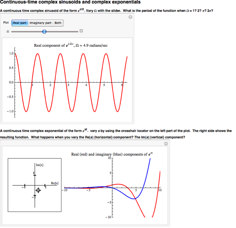
It has been shown how the complex exponential with purely imaginary frequency can be broken up into its real part and its imaginary part. Now consider a general complex frequency \(s=\sigma+\omega j\) where \(\sigma\) is the attenuation factor and \(\omega\) is the frequency. Also consider a phase difference \(\theta\). It follows that
\[e^{(\sigma+j \omega) t+j \theta}=e^{\sigma t}(\cos (\omega t+\theta)+j \sin (\omega t+\theta)) \nonumber \]
Thus, the real and imaginary parts of \(e^{st}\) appear below.
\[\operatorname{Re}\left\{e^{(\sigma+j \omega) t+j \theta}\right\}=e^{\sigma t} \cos (\omega t+\theta) \nonumber \]
\[\operatorname{Im}\left\{e^{(\sigma+j \omega) t+j \theta}\right\}=e^{\sigma t} \sin (\omega t+\theta) \nonumber \]
Using the real or imaginary parts of complex exponential to represent sinusoids with a phase delay multiplied by real exponential is often useful and is called attenuated phasor notation.
We can see that both the real part and the imaginary part have a sinusoid times a real exponential. We also know that sinusoids oscillate between one and negative one. From this it becomes apparent that the real and imaginary parts of the complex exponential will each oscillate within an envelope defined by the real exponential part.
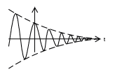 (a)
(a)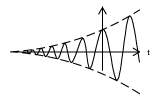 (b)
(b)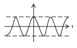 (c)
(c)Complex Exponential Demonstration
Continuous Time Complex Exponential Summary
Continuous time complex exponentials are signals of great importance to the study of signals and systems. They can be related to sinusoids through Euler's formula, which identifies the real and imaginary parts of purely imaginary complex exponentials. Eulers formula reveals that, in general, the real and imaginary parts of complex exponentials are sinusoids multiplied by real exponentials. Thus, attenuated phasor notation is often useful in studying these signals.