
1.9: Discrete Time Complex Exponential
- Page ID
- 23115

Introduction
Complex exponentials are some of the most important functions in our study of signals and systems. Their importance stems from their status as eigenfunctions of linear time invariant systems; as such, it can be both convenient and insightful to represent signals in terms of complex exponentials. Before proceeding, you should be familiar with complex numbers.
The Discrete Time Complex Exponential
Complex Exponentials
The complex exponential function will become a critical part of your study of signals and systems. Its general discrete form is written as
\[z^n \nonumber \]
where \(z\) is a complex number. Recalling the polar expression of complex numbers, \(z\) can be expressed in terms of its magnitude \(|z|\) and its angle (or argument) \(\omega\) in the complex plane: \(z=|z| e^{j \omega}\). Thus \(z^{n}=(|z|)^{n} e^{j \omega n}\). In the context of complex exponentials, \(\omega\) is referred to as frequency. For the time being, let's consider complex exponentials for which \(|z|=1\).
These discrete time complex exponentials have the following property, which will become evident through discussion of Euler's formula.
\[e^{j \omega n}=e^{j(\omega+2 \pi) n} \nonumber \]
Given this property, if we have a complex exponential with frequency \(\omega + 2 \pi\), then this signal "aliases" to a complex exponential with frequency \(\omega\), implying that the equation representations of discrete complex exponentials are not unique.
Euler's Formula
The mathematician Euler proved an important identity relating complex exponentials to trigonometric functions. Specifically, he discovered the eponymously named identity, Euler's formula, which states that for any real number \(x\),
\[e^{j x}=\cos (x)+j \sin (x) \nonumber \]
which can be proven as follows.
In order to prove Euler's formula, we start by evaluating the Taylor series for \(e^z\) about \(z=0\), which converges for all complex \(z\), at \(z=jx\). The result is
\begin{align}
e^{j x} &=\sum_{k=0}^{\infty} \frac{(j x)^{k}}{k !} \nonumber \\
&=\sum_{k=0}^{\infty}(-1)^{k} \frac{x^{2 k}}{(2 k) !}+j \sum_{k=0}^{\infty}(-1)^{k} \frac{x^{2 k+1}}{(2 k+1) !} \nonumber \\
&=\cos (x)+j \sin (x)
\end{align}
because the second expression contains the Taylor series for \(\cos(x)\) and \(\sin(x)\) about \(t=0\), which converge for all real \(x\). Thus, the desired result is proven.
Choosing \(x=\omega n\), we have:
\[e^{j \omega n}=\cos (\omega n)+j \sin (\omega n) \nonumber \]
which breaks a discrete time complex exponential into its real part and imaginary part. Using this formula, we can also derive the following relationships.
\[\cos (\omega n)=\frac{1}{2} e^{j \omega n}+\frac{1}{2} e^{-j \omega n} \nonumber \]
\[\sin (\omega n)=\frac{1}{2 j} e^{j \omega n}-\frac{1}{2 j} e^{-j \omega n} \nonumber \]
Real and Imaginary Parts of Complex Exponentials
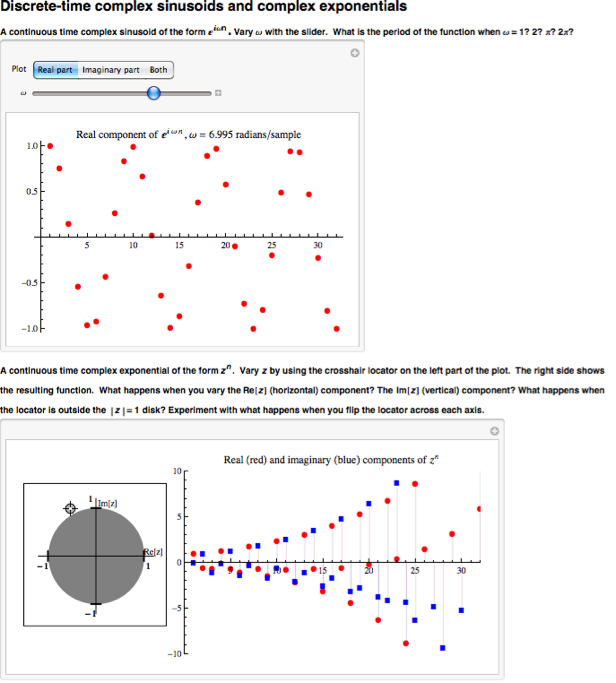
Now let's return to the more general case of complex exponentials, \(z^n\). Recall that \(z^{n}=(|z|)^{n} e^{j \omega n}\). We can express this in terms of its real and imaginary parts:
\[\operatorname{Re}\left\{z^{n}\right\}=(|z|)^{n} \cos (\omega n) \nonumber \]
\[\operatorname{Im}\left\{z^{n}\right\}=(|z|)^{n} \sin (\omega n) \nonumber \]
We see now that the magnitude of \(z\) establishes an exponential envelope to the signal, with \(\omega\) controlling rate of the sinusoidal oscillation within the envelope.
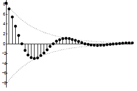 (a)
(a)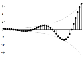 (b)
(b)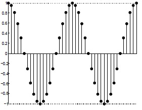 (c)
(c)
Discrete Complex Exponential Demonstration
Discrete Time Complex Exponential Summary
Discrete time complex exponentials are signals of great importance to the study of signals and systems. They can be related to sinusoids through Euler's formula, which identifies the real and imaginary parts of complex exponentials. Eulers formula reveals that, in general, the real and imaginary parts of complex exponentials are sinusoids multiplied by real exponentials.