3.1: Continuous Time Systems

Last updated
Save as PDF

Page ID: 22851

\( \newcommand{\vecs}[1]{\overset { \scriptstyle \rightharpoonup} {\mathbf{#1}} } \) \( \newcommand{\vecd}[1]{\overset{-\!-\!\rightharpoonup}{\vphantom{a}\smash {#1}}} \)\(\newcommand{\id}{\mathrm{id}}\) \( \newcommand{\Span}{\mathrm{span}}\) \( \newcommand{\kernel}{\mathrm{null}\,}\) \( \newcommand{\range}{\mathrm{range}\,}\) \( \newcommand{\RealPart}{\mathrm{Re}}\) \( \newcommand{\ImaginaryPart}{\mathrm{Im}}\) \( \newcommand{\Argument}{\mathrm{Arg}}\) \( \newcommand{\norm}[1]{\| #1 \|}\) \( \newcommand{\inner}[2]{\langle #1, #2 \rangle}\) \( \newcommand{\Span}{\mathrm{span}}\) \(\newcommand{\id}{\mathrm{id}}\) \( \newcommand{\Span}{\mathrm{span}}\) \( \newcommand{\kernel}{\mathrm{null}\,}\) \( \newcommand{\range}{\mathrm{range}\,}\) \( \newcommand{\RealPart}{\mathrm{Re}}\) \( \newcommand{\ImaginaryPart}{\mathrm{Im}}\) \( \newcommand{\Argument}{\mathrm{Arg}}\) \( \newcommand{\norm}[1]{\| #1 \|}\) \( \newcommand{\inner}[2]{\langle #1, #2 \rangle}\) \( \newcommand{\Span}{\mathrm{span}}\)\(\newcommand{\AA}{\unicode[.8,0]{x212B}}\)

Introduction

As you already now know, a continuous time system operates on a continuous time signal input and produces a continuous time signal output. There are numerous examples of useful continuous time systems in signal processing as they essentially describe the world around us. The class of continuous time systems that are both linear and time invariant, known as continuous time LTI systems, is of particular interest as the properties of linearity and time invariance together allow the use of some of the most important and powerful tools in signal processing.

Continuous Time Systems

Linearity and Time Invariance

A system \(H\) is said to be linear if it satisfies two important conditions. The first, additivity, states for every pair of signals \(x\), \(y\) that \(H(x+y)=H(x)+H(y)\). The second, homogeneity of degree one, states for every signal \(x\) and scalar \(a\) we have \(H(ax)=aH(x)\). It is clear that these conditions can be combined together into a single condition for linearity. Thus, a system is said to be linear if for every signals \(x\), \(y\) and scalars \(a\), \(b\) we have that

\[H(a x+b y)=a H(x)+b H(y) \nonumber \]

Linearity is a particularly important property of systems as it allows us to leverage the powerful tools of linear algebra, such as bases, eigenvectors, and eigenvalues, in their study.

A system \(H\) is said to be time invariant if a time shift of an input produces the corresponding shifted output. In other, more precise words, the system \(H\) commutes with the time shift operator \(S_T\) for every \(T \in \mathbb{R}\). That is,

\[S_{T} H=H S_{T} \nonumber \]

Time invariance is desirable because it eases computation while mirroring our intuition that, all else equal, physical systems should react the same to identical inputs at different times.

When a system exhibits both of these important properties it allows for a more straigtforward analysis than would otherwise be possible. As will be explained and proven in subsequent modules, computation of the system output for a given input becomes a simple matter of convolving the input with the system's impulse response signal. Also proven later, the fact that complex exponential are eigenvectors of linear time invariant systems will enable the use of frequency domain tools such as the various Fourier transforms and associated transfer functions, to describe the behavior of linear time invariant systems.

Example \(\PageIndex{1}\)

Consider the system \(H\) in which

\[H(f(t))=2 f(t) \nonumber \]

for all signals \(f\). Given any two signals \(f\), \(g\) and scalars \(a\), \(b\)

\[H(a f(t)+b g(t)))=2(a f(t)+b g(t))=a 2 f(t)+b 2 g(t)=a H(f(t))+b H(g(t)) \nonumber \]

for all real \(t\). Thus, \(H\) is a linear system. For all real \(T\) and signals \(f\),

\[S_{T}(H(f(t)))=S_{T}(2 f(t))=2 f(t-T)=H(f(t-T))=H\left(S_{T}(f(t))\right) \nonumber \]

for all real \(t\). Thus, \(H\) is a time invariant system. Therefore, \(H\) is a linear time invariant system.

Differential Equation Representation

It is often useful to to describe systems using equations involving the rate of change in some quantity. For continuous time systems, such equations are called differential equations. One important class of differential equations is the set of linear constant coefficient ordinary differential equations, which are described in more detail in subsequent modules.

Example \(\PageIndex{2}\)

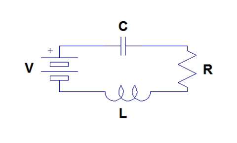
Consider the series RLC circuit shown in Figure \(\PageIndex{1}\). This system can be modeled using differential equations. We can use the voltage equations for each circuit element and Kirchoff's voltage law to write a second order linear constant coefficient differential equation describing the charge on the capacitor.

The voltage across the battery is simply \(V\). The voltage across the capacitor is \(\frac{1}{C}q\). The voltage across the resistor is \(R\frac{dq}{dt}\). Finally, the voltage across the inductor is \(L \frac{d^{2} q}{d t^{2}}\). Therefore, by Kirchoff's voltage law, it follows that

\[L \frac{d^{2} q}{d t^{2}}+R \frac{d q}{d t}+\frac{1}{C} q=V \nonumber \]

Figure \(\PageIndex{1}\): A series RLC circuit.

Continuous Time Systems Summary

Many useful continuous time systems will be encountered in a study of signals and systems. This course is most interested in those that demonstrate both the linearity property and the time invariance property, which together enable the use of some of the most powerful tools of signal processing. It is often useful to describe them in terms of rates of change through linear constant coefficient ordinary differential equations.