Engineering LibreTexts

3.2: Continuous Time Impulse Response

  • Page ID
    22852
  • \( \newcommand{\vecs}[1]{\overset { \scriptstyle \rightharpoonup} {\mathbf{#1}} } \) \( \newcommand{\vecd}[1]{\overset{-\!-\!\rightharpoonup}{\vphantom{a}\smash {#1}}} \)\(\newcommand{\id}{\mathrm{id}}\) \( \newcommand{\Span}{\mathrm{span}}\) \( \newcommand{\kernel}{\mathrm{null}\,}\) \( \newcommand{\range}{\mathrm{range}\,}\) \( \newcommand{\RealPart}{\mathrm{Re}}\) \( \newcommand{\ImaginaryPart}{\mathrm{Im}}\) \( \newcommand{\Argument}{\mathrm{Arg}}\) \( \newcommand{\norm}[1]{\| #1 \|}\) \( \newcommand{\inner}[2]{\langle #1, #2 \rangle}\) \( \newcommand{\Span}{\mathrm{span}}\) \(\newcommand{\id}{\mathrm{id}}\) \( \newcommand{\Span}{\mathrm{span}}\) \( \newcommand{\kernel}{\mathrm{null}\,}\) \( \newcommand{\range}{\mathrm{range}\,}\) \( \newcommand{\RealPart}{\mathrm{Re}}\) \( \newcommand{\ImaginaryPart}{\mathrm{Im}}\) \( \newcommand{\Argument}{\mathrm{Arg}}\) \( \newcommand{\norm}[1]{\| #1 \|}\) \( \newcommand{\inner}[2]{\langle #1, #2 \rangle}\) \( \newcommand{\Span}{\mathrm{span}}\)\(\newcommand{\AA}{\unicode[.8,0]{x212B}}\)

    Introduction

    The output of an LTI system is completely determined by the input and the system's response to a unit impulse.

    System Output A continuous time system H takes the input f(t) and produces the output y(t).
    Figure \(\PageIndex{1}\): We can determine the system's output, \(y(t)\), if we know the system's impulse response, \(h(t)\), and the input, \(f(t)\).

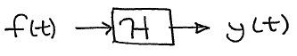
    The output for a unit impulse input is called the impulse response.

    An impulse input delta(t) going through a continuous time system H, producing the system's impulse response, h(t). delta(t) 'shocks' the system suddenly and h(t) is the response to the shock.

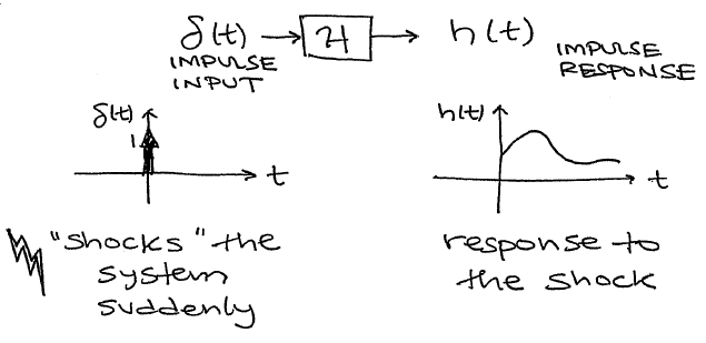
    Figure \(\PageIndex{2}\)

    Example Approximate Impulses

    1. Hammer blow to a structure
    2. Hand clap or gun blast in a room
    3. Air gun blast underwater

    LTI Systems and Impulse Responses

    Finding System Outputs

    By the sifting property of impulses, any signal can be decomposed in terms of an integral of shifted, scaled impulses.

    \[f(t)=\int_{-\infty}^{\infty} f(\tau) \delta(t-\tau) \mathrm{d} \tau \nonumber \]

    \(\delta(t-\tau)\) peaks up where \(t=\tau\).

    The functions δ(t-τ) and f(τ) as functions of τ. δ(t-τ) is a peak of infinite height and zero width at point t. f(τ) is some function with a strange shape. Point t is marked on the graphs of both of them.

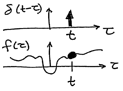
    Figure \(\PageIndex{3}\)

    Since we know the response of the system to an impulse and any signal can be decomposed into impulses, all we need to do to find the response of the system to any signal is to decompose the signal into impulses, calculate the system's output for every impulse and add the outputs back together. This is the process known as Convolution. Since we are in Continuous Time, this is the Continuous Time Convolution Integral.

    Finding Impulse Responses

    Theory:

    1. Solve the system's differential equation for \(y(t)\) with \(f(t)=\delta(t)\)
    2. Use the Laplace transform

    Practice:

    1. Apply an impulse-like input signal to the system and measure the output
    2. Use Fourier methods

    We will assume that \(h(t)\) is given for now.

    • The goal now is to compute the output \(y(t)\) given the impulse response \(h(t)\) and the input \(f(t)\).
    A system with impulse response h takes the input f and produces the output y.

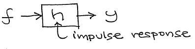
    Figure \(\PageIndex{4}\)

    Impulse Response Summary

    When a system is "shocked" by a delta function, it produces an output known as its impulse response. For an LTI system, the impulse response completely determines the output of the system given any arbitrary input. The output can be found using continuous time convolution.


    This page titled 3.2: Continuous Time Impulse Response is shared under a CC BY license and was authored, remixed, and/or curated by Richard Baraniuk et al..

    • Was this article helpful?