
6.6: Convergence of Fourier Series
- Page ID
- 22877

\( \newcommand{\vecs}[1]{\overset { \scriptstyle \rightharpoonup} {\mathbf{#1}} } \)
\( \newcommand{\vecd}[1]{\overset{-\!-\!\rightharpoonup}{\vphantom{a}\smash {#1}}} \)
\( \newcommand{\dsum}{\displaystyle\sum\limits} \)
\( \newcommand{\dint}{\displaystyle\int\limits} \)
\( \newcommand{\dlim}{\displaystyle\lim\limits} \)
\( \newcommand{\id}{\mathrm{id}}\) \( \newcommand{\Span}{\mathrm{span}}\)
( \newcommand{\kernel}{\mathrm{null}\,}\) \( \newcommand{\range}{\mathrm{range}\,}\)
\( \newcommand{\RealPart}{\mathrm{Re}}\) \( \newcommand{\ImaginaryPart}{\mathrm{Im}}\)
\( \newcommand{\Argument}{\mathrm{Arg}}\) \( \newcommand{\norm}[1]{\| #1 \|}\)
\( \newcommand{\inner}[2]{\langle #1, #2 \rangle}\)
\( \newcommand{\Span}{\mathrm{span}}\)
\( \newcommand{\id}{\mathrm{id}}\)
\( \newcommand{\Span}{\mathrm{span}}\)
\( \newcommand{\kernel}{\mathrm{null}\,}\)
\( \newcommand{\range}{\mathrm{range}\,}\)
\( \newcommand{\RealPart}{\mathrm{Re}}\)
\( \newcommand{\ImaginaryPart}{\mathrm{Im}}\)
\( \newcommand{\Argument}{\mathrm{Arg}}\)
\( \newcommand{\norm}[1]{\| #1 \|}\)
\( \newcommand{\inner}[2]{\langle #1, #2 \rangle}\)
\( \newcommand{\Span}{\mathrm{span}}\) \( \newcommand{\AA}{\unicode[.8,0]{x212B}}\)
\( \newcommand{\vectorA}[1]{\vec{#1}} % arrow\)
\( \newcommand{\vectorAt}[1]{\vec{\text{#1}}} % arrow\)
\( \newcommand{\vectorB}[1]{\overset { \scriptstyle \rightharpoonup} {\mathbf{#1}} } \)
\( \newcommand{\vectorC}[1]{\textbf{#1}} \)
\( \newcommand{\vectorD}[1]{\overrightarrow{#1}} \)
\( \newcommand{\vectorDt}[1]{\overrightarrow{\text{#1}}} \)
\( \newcommand{\vectE}[1]{\overset{-\!-\!\rightharpoonup}{\vphantom{a}\smash{\mathbf {#1}}}} \)
\( \newcommand{\vecs}[1]{\overset { \scriptstyle \rightharpoonup} {\mathbf{#1}} } \)
\(\newcommand{\longvect}{\overrightarrow}\)
\( \newcommand{\vecd}[1]{\overset{-\!-\!\rightharpoonup}{\vphantom{a}\smash {#1}}} \)
\(\newcommand{\avec}{\mathbf a}\) \(\newcommand{\bvec}{\mathbf b}\) \(\newcommand{\cvec}{\mathbf c}\) \(\newcommand{\dvec}{\mathbf d}\) \(\newcommand{\dtil}{\widetilde{\mathbf d}}\) \(\newcommand{\evec}{\mathbf e}\) \(\newcommand{\fvec}{\mathbf f}\) \(\newcommand{\nvec}{\mathbf n}\) \(\newcommand{\pvec}{\mathbf p}\) \(\newcommand{\qvec}{\mathbf q}\) \(\newcommand{\svec}{\mathbf s}\) \(\newcommand{\tvec}{\mathbf t}\) \(\newcommand{\uvec}{\mathbf u}\) \(\newcommand{\vvec}{\mathbf v}\) \(\newcommand{\wvec}{\mathbf w}\) \(\newcommand{\xvec}{\mathbf x}\) \(\newcommand{\yvec}{\mathbf y}\) \(\newcommand{\zvec}{\mathbf z}\) \(\newcommand{\rvec}{\mathbf r}\) \(\newcommand{\mvec}{\mathbf m}\) \(\newcommand{\zerovec}{\mathbf 0}\) \(\newcommand{\onevec}{\mathbf 1}\) \(\newcommand{\real}{\mathbb R}\) \(\newcommand{\twovec}[2]{\left[\begin{array}{r}#1 \\ #2 \end{array}\right]}\) \(\newcommand{\ctwovec}[2]{\left[\begin{array}{c}#1 \\ #2 \end{array}\right]}\) \(\newcommand{\threevec}[3]{\left[\begin{array}{r}#1 \\ #2 \\ #3 \end{array}\right]}\) \(\newcommand{\cthreevec}[3]{\left[\begin{array}{c}#1 \\ #2 \\ #3 \end{array}\right]}\) \(\newcommand{\fourvec}[4]{\left[\begin{array}{r}#1 \\ #2 \\ #3 \\ #4 \end{array}\right]}\) \(\newcommand{\cfourvec}[4]{\left[\begin{array}{c}#1 \\ #2 \\ #3 \\ #4 \end{array}\right]}\) \(\newcommand{\fivevec}[5]{\left[\begin{array}{r}#1 \\ #2 \\ #3 \\ #4 \\ #5 \\ \end{array}\right]}\) \(\newcommand{\cfivevec}[5]{\left[\begin{array}{c}#1 \\ #2 \\ #3 \\ #4 \\ #5 \\ \end{array}\right]}\) \(\newcommand{\mattwo}[4]{\left[\begin{array}{rr}#1 \amp #2 \\ #3 \amp #4 \\ \end{array}\right]}\) \(\newcommand{\laspan}[1]{\text{Span}\{#1\}}\) \(\newcommand{\bcal}{\cal B}\) \(\newcommand{\ccal}{\cal C}\) \(\newcommand{\scal}{\cal S}\) \(\newcommand{\wcal}{\cal W}\) \(\newcommand{\ecal}{\cal E}\) \(\newcommand{\coords}[2]{\left\{#1\right\}_{#2}}\) \(\newcommand{\gray}[1]{\color{gray}{#1}}\) \(\newcommand{\lgray}[1]{\color{lightgray}{#1}}\) \(\newcommand{\rank}{\operatorname{rank}}\) \(\newcommand{\row}{\text{Row}}\) \(\newcommand{\col}{\text{Col}}\) \(\renewcommand{\row}{\text{Row}}\) \(\newcommand{\nul}{\text{Nul}}\) \(\newcommand{\var}{\text{Var}}\) \(\newcommand{\corr}{\text{corr}}\) \(\newcommand{\len}[1]{\left|#1\right|}\) \(\newcommand{\bbar}{\overline{\bvec}}\) \(\newcommand{\bhat}{\widehat{\bvec}}\) \(\newcommand{\bperp}{\bvec^\perp}\) \(\newcommand{\xhat}{\widehat{\xvec}}\) \(\newcommand{\vhat}{\widehat{\vvec}}\) \(\newcommand{\uhat}{\widehat{\uvec}}\) \(\newcommand{\what}{\widehat{\wvec}}\) \(\newcommand{\Sighat}{\widehat{\Sigma}}\) \(\newcommand{\lt}{<}\) \(\newcommand{\gt}{>}\) \(\newcommand{\amp}{&}\) \(\definecolor{fillinmathshade}{gray}{0.9}\)Introduction
Before looking at this module, hopefully you have become fully convinced of the fact that any periodic function, \(f(t)\), can be represented as a sum of complex sinusoids (Section 1.4). If you are not, then try looking back at eigen-stuff in a nutshell (Section 14.4) or eigenfunctions of LTI systems (Section 14.5). We have shown that we can represent a signal as the sum of exponentials through the Fourier Series equations below:
\[f(t)=\sum_{n} c_{n} e^{j \omega_{0} n t} \label{6.35} \]
\[c_{n}=\frac{1}{T} \int_{0}^{T} f(t) e^{-\left(j \omega_{0} n t\right)} d t \label{6.36} \]
Joseph Fourier insisted that these equations were true, but could not prove it. Lagrange publicly ridiculed Fourier, and said that only continuous functions can be represented by Equation \ref{6.35} (indeed he proved that Equation \ref{6.35} holds for continuous-time functions). However, we know now that the real truth lies in between Fourier and Lagrange's positions.
Understanding the Truth
Formulating our question mathematically, let
\[f_{N}^{\prime}(t)=\sum_{n=-N}^{N} c_{n} e^{j \omega_{0} n t} \nonumber \]
where \(c_n\) equals the Fourier coefficients of \(f(t)\) (see Equation \ref{6.36}).
\(f_{N}^{\prime}(t)\) is a "partial reconstruction" of \(f(t)\) using the first \(2N+1\) Fourier coefficients. \(f_{N}^{\prime}\) approximates \(f(t)\), with the approximation getting better and better as \(N\) gets large. Therefore, we can think of the set \(\left\{\forall N, N=\{0,1, \ldots\}:\left(\frac{\mathrm{d} f_{N}(t)}{\mathrm{d}}\right)\right\}\) as a sequence of functions, each one approximating \(f(t)\) better than the one before.
The question is, does this sequence converge to \(f(t)\)? Does \( f_{N}^{\prime}(t) \rightarrow f(t)\) as \(N \rightarrow \infty\)? We will try to answer this question by thinking about convergence in two different ways:
- Looking at the energy of the error signal:
\[e_{N}(t)=f(t)-f_{N}^{\prime}(t) \nonumber \]
- Looking at \(\displaystyle{\lim_{N \to \infty}} \frac{d f_{N}(t)}{d}\) at each point and comparing to \(f(t)\).
Approach #1
Let \(e_N(t)\) be the difference (i.e. error) between the signal \(f(t)\) and its partial reconstruction \(f_N^{\prime}\)
\[e_{N}(t)=f(t)-f_{N}^{\prime}(t) \nonumber \]
If \(f(t) \in L^{2}([0, T])\) (finite energy), then the energy of \(e_{N}(t) \rightarrow 0\) as \(N \rightarrow \infty\) is
\[\int_{0}^{T}\left(\left|e_{N}(t)\right|\right)^{2} \mathrm{d} t=\int_{0}^{T}\left(f(t)-f_{N}^{\prime}(t)\right)^{2} \mathrm{d} t \rightarrow 0 \nonumber \]
We can prove this equation using Parseval's relation:
\[\lim_{N \rightarrow \infty} \int_{0}^{T}\left(\left|f(t)-f_{N}^{\prime}(t)\right|\right)^{2} \mathrm{d} t=\lim_{N \rightarrow \infty} \sum_{N=-\infty}^{\infty}\left(\left|\mathscr{F}_{n}(f(t))-\mathscr{F}_{n}\left(\frac{\mathrm{d} f_{N}(t)}{\mathrm{d}}\right)\right|\right)^{2}=\lim_{N \rightarrow \infty} \sum_{|n|>N}\left(\left|c_{n}\right|\right)^{2}=0 \nonumber \]
where the last equation before zero is the tail sum of the Fourier Series, which approaches zero because \(f(t) \in L^{2}([0, T])\). Since physical systems respond to energy, the Fourier Series provides an adequate representation for all \(f(t) \in L^{2}([0, T])\) equaling finite energy over one period.
Approach #2
The fact that \(e_{N} \rightarrow 0\) says nothing about \(f(t)\) and \(\displaystyle{\lim_{N \rightarrow \infty}} \frac{\mathrm{d} f_{N}(t)}{\mathrm{d}}\) being equal at a given point. Take the two functions graphed below for example:
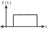 (a)
(a)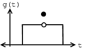 (b)
(b)
Figure \(\PageIndex{1}\)
Given these two functions, \(f(t)\) and \(g(t)\), then we can see that for all \(t\), \(f(t) \neq g(t)\), but
\[\int_{0}^{T}(|f(t)-g(t)|)^{2} \mathrm{d} t=0 \nonumber \]
From this we can see the following relationships:
energy convergence \(\neq\) pointwise convergence
pointwise convergence \(\Rightarrow\) convergence in \(L^2([0,T])\)
However, the reverse of the above statement does not hold true.
It turns out that if \(f(t)\) has a discontinuity (as can be seen in figure of \(g(t)\) above) at \(t_0\), then
\[f\left(t_{0}\right) \neq \lim_{N \rightarrow \infty} \frac{\mathrm{d} f_{N}\left(t_{0}\right)}{\mathrm{d}} \nonumber \]
But as long as \(f(t)\) meets some other fairly mild conditions, then
\[f\left(t^{\prime}\right)=\lim_{N \rightarrow \infty} \frac{\left.\mathrm{d} f_{N}\left(t^{\prime}\right)\right)}{\mathrm{d}} \nonumber \]
if \(f(t)\) is continuous at \(t=t^{\prime}\).
These conditions are known as the Dirichlet Conditions.
Dirichlet Conditions
Named after the German mathematician, Peter Dirichlet, the Dirichlet conditions are the sufficient conditions to guarantee existence and energy convergence of the Fourier Series.
The Weak Dirichlet Condition for the Fourier Series
For the Fourier Series to exist, the Fourier coefficients must be finite. The Weak Dirichlet Condition guarantees this. It essentially says that the integral of the absolute value of the signal must be finite.
Theorem \(\PageIndex{1}\): Weak Dirichlet Condition for the Fourier Series
The coefficients of the Fourier Series are finite if
\[\int_{0}^{T}|f(t)| d t<\infty \nonumber \]
Proof
This can be shown from the magnitude of the Fourier Series coefficients:
\[\left|c_{n}\right|=\left|\frac{1}{T} \int_{0}^{T} f(t) e^{-\left(j \omega_{0} n t\right)} d t\right| \leq \frac{1}{T} \int_{0}^{T}\left|f(t) \| e^{-\left(j \omega_{0} n t\right)}\right| d t \nonumber \]
Remembering our complex exponentials (Section 1.8), we know that in the above equation \(\left|e^{-\left(j \omega_{0} n t\right)}\right|=1\), which gives us:
\[\begin{align}
\left|c_{n}\right| \leq & \frac{1}{T} \int_{0}^{T}|f(t)| d t<\infty \\
& \Rightarrow\left(\left|c_{n}\right|<\infty\right)
\end{align} \nonumber \]
Note
If we have the function:
\[\forall t, 0<t \leq T:\left(f(t)=\frac{1}{t}\right) \nonumber \]
then you should note that this function fails the above condition because:
\[\int_{0}^{T}\left|\frac{1}{t}\right| \mathrm{d} t=\infty \nonumber \]
The Strong Dirichlet Conditions for the Fourier Series
For the Fourier Series to exist, the following two conditions must be satisfied (along with the Weak Dirichlet Condition):
- In one period, \(f(t)\) has only a finite number of minima and maxima.
- In one period, \(f(t)\) has only a finite number of discontinuities and each one is finite.
These are what we refer to as the Strong Dirichlet Conditions. In theory we can think of signals that violate these conditions, \(\sin(\log t)\) for instance. However, it is not possible to create a signal that violates these conditions in a lab. Therefore, any real-world signal will have a Fourier representation.
Example \(\PageIndex{1}\)
Let us assume we have the following function and equality:
\[f^{\prime}(t)=\lim_{N \rightarrow \infty} \frac{\mathrm{d} f_{N}(t)}{\mathrm{d}} \nonumber \]
If \(f(t)\) meets all three conditions of the Strong Dirichlet Conditions, then
\[f(\tau)=f^{\prime}(\tau) \nonumber \]
at every \(\tau\) at which \(f(t)\) is continuous. And where \(f(t)\) is discontinuous, \(f^{\prime}(t)\) is the average of the values on the right and left.
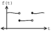 (a)
(a)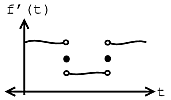 (b)
(b)Note
The functions that fail the strong Dirchlet conditions are pretty pathological - as engineers, we are not too interested in them.