2.7: Exercises

Exercise 2.1

1. Find the Erlang density \(\mathrm{f}_{S_{n}}(t)\) by convolving \(\mathrm{f}_{X}(x)=\lambda \exp (-\lambda x)\) with itself \(n\) times.
2. Find the moment generating function of \(X\) (or find the Laplace transform of \(f_{X}(x)\)), and use this to find the moment generating function (or Laplace transform) of \(S_{n}=X_{1}+X_{2}+\dots+X_n\). Invert your result to find \(\mathrm{f}_{S_{n}}(t)\).
3. Find the Erlang density by starting with \ref{2.15} and then calculating the marginal density for \(S_{n}\).

Answer

Exercise 2.2

1. Find the mean, variance, and moment generating function of \(N(t)\), as given by (2.16).
2. Show by discrete convolution that the sum of two independent Poisson rv’s is again Poisson.
3. Show by using the properties of the Poisson process that the sum of two independent Poisson rv’s must be Poisson.

Answer

Exercise 2.3

The purpose of this exercise is to give an alternate derivation of the Poisson distribution for \(N(t)\), the number of arrivals in a Poisson process up to time \(t\). Let \(\lambda\) be the rate of the process.

1. Find the conditional probability \(\operatorname{Pr}\left\{N(t)=n \mid S_{n}=\tau\right\}\) for all \(\tau \leq t\).
2. Using the Erlang density for \(S_{n}\), use \ref{a} to find \(\operatorname{Pr}\{N(t)=n\}\).

Answer

Exercise 2.4

Assume that a counting process \(\{N(t) ; t>0\}\) has the independent and stationary increment properties and satisfies \ref{2.16} (for all \(t>0\)). Let \(X_{1}\) be the epoch of the first arrival and \(X_{n}\) be the interarrival time between the \(n-1^{\mathrm{st}}\) and the \(n\)th arrival. Use only these assumptions in doing the following parts of this exercise.

1. Show that \(\operatorname{Pr}\left\{X_{1}>x\right\}=e^{-\lambda x}\).
2. Let \(S_{n-1}\) be the epoch of the \(n-1^{\mathrm{st}}\) arrival. Show that \(\operatorname{Pr}\left\{X_{n}>x \mid S_{n-1}=\tau\right\}=e^{-\lambda x}\).
3. For each \(n>1\), show that \(\operatorname{Pr}\left\{X_{n}>x\right\}=e^{-\lambda x}\) and that \(X_{n}\) is independent of \(S_{n-1}\).
4. Argue that \(X_{n}\) is independent of \(X_{1}, X_{2}, \ldots X_{n-1}\).

Answer

Exercise 2.5

The point of this exercise is to show that the sequence of PMF’s for a Bernoulli counting process does not specify the process. In other words, knowing that \(N(t)\) satisfies the binomial distribution for all \(t\) does not mean that the process is Bernoulli. This helps us understand why the second definition of a Poisson process requires stationary and independent increments as well as the Poisson distribution for \(N(t)\).

1. Let \(Y_{1}, Y_{2}, Y_{3}, \ldots\) be a sequence of binary rv’s in which each rv is 0 or 1 with equal probability. Find a joint distribution for \(Y_{1}, Y_{2}, Y_{3}\) that satisfies the binomial distribution, \(\mathbf{p}_{N(t)}(k)=\left(\begin{array}{l} t \\ k \end{array}\right) 2^{-k}\) for \(t=1,2,3\) and \(0 \leq k \leq t\), but for which \(Y_{1}, Y_{2}, Y_{3}\) are not independent.

   One simple solution for this contains four 3-tuples with probability 1/8 each, two 3-tuples with probability 1/4 each, and two 3-tuples with probability 0. Note that by making the subsequent arrivals IID and equiprobable, you have an example where \(N(t)\) is binomial for all t but the process is not Bernoulli. Hint: Use the binomial for \(t=3\) to find two 3-tuples that must have probability 1/8. Combine this with the binomial for \(t=2\) to find two other 3-tuples that must have probability 1/8. Finally look at the constraints imposed by the binomial distribution on the remaining four 3-tuples.

2. Generalize part a) to the case where \(Y_{1}, Y_{2}, Y_{3}\) satisfy \(\operatorname{Pr}\left\{Y_{i}=1\right\}=p\) and \(\operatorname{Pr}\left\{Y_{i}=0\right\}=1-p\). Assume \(p<1 / 2\) and find a joint distribution on \(Y_{1}, Y_{2}, Y_{3}\) that satisfies the binomial distribution, but for which the 3-tuple (0, 1, 1) has zero probability.
3. More generally yet, view a joint PMF on binary \(t\)-tuples as a nonnegative vector in a \(2^{t}\) dimensional vector space. Each binomial probability \(\mathbf{p}_{N(\tau)}(k)=\left(\begin{array}{l} \tau \\ k \end{array}\right) p^{k}(1-p)^{\tau-k}\) constitutes a linear constraint on this vector. For each \(\tau\), show that one of these constraints may be replaced by the constraint that the components of the vector sum to 1.
4. Using part c), show that at most \((t+1) t / 2+1\) of the binomial constraints are linearly independent. Note that this means that the linear space of vectors satisfying these binomial constraints has dimension at least \(2^{t}-(t+1) t / 2-1\). This linear space has dimension 1 for \(t=3\), explaining the results in parts a) and b). It has a rapidly increasing dimension for \(t>3\), suggesting that the binomial constraints are relatively ineffectual for constraining the joint PMF of a joint distribution. More work is required for the case of \(t>3\) because of all the inequality constraints, but it turns out that this large dimensionality remains.

Answer

Exercise 2.6

Let \(h(x)\) be a positive function of a real variable that satisfies \(h(x+t)=h(x)+h(t)\) and let \(h(1)=c\).

1. Show that for integer \(k>0, h(k)=k c\).
2. Show that for integer \(j>0, h(1 / j)=c / j\).
3. Show that for all integer \(k, j, h(k / j)=c k / j\).
4. The above parts show that \(h(x)\) is linear in positive rational numbers. For very picky mathematicians, this does not guarantee that \(h(x)\) is linear in positive real numbers. Show that if \(h(x)\) is also monotonic in \(x\), then \(h(x)\) is linear in \(x>0\).

Answer

Exercise 2.7

Assume that a counting process \(\{N(t) ; t>0\}\) has the independent and sta­tionary increment properties and, for all \(t>0\), satisfies

\(\begin{aligned}
&\operatorname{Pr}\{\tilde{N}(t, t+\delta)=0\}^\}=1-\lambda \delta+o(\delta) \\
&\operatorname{Pr}\{\widetilde{N}(t, t+\delta)=1\}^\}=\lambda \delta+o(\delta) \\
&\operatorname{Pr}\{\widetilde{N}(t, t+\delta)>1\}^\}=o(\delta)
\end{aligned}\)

1. Let \(\mathrm{F}_{0}(\tau)=\operatorname{Pr}\{N(\tau)=0\}\) and show that \(d \mathrm{~F}_{0}(\tau) / d \tau=-\lambda \mathrm{F}_{0}(\tau)\).
2. Show that \(X_{1}\), the time of the first arrival, is exponential with parameter \(\lambda\).
3. Let \(\mathrm{F}_{n}(\tau)=\operatorname{Pr}\left\{\tilde{N}(t, t+\tau)=0 \mid S_{n-1}=t\right\}^\}\) and show that \(d \mathrm{~F}_{n}(\tau) / d \tau=-\lambda \mathrm{F}_{n}(\tau)\).
4. Argue that \(X_{n}\) is exponential with parameter \(\lambda\) and independent of earlier arrival times.

Answer

Exercise 2.8

Let \(t>0\) be an arbitrary time, let \(Z_{1}\) be the duration of the interval from \(t\) until the next arrival after \(t\). Let \(Z_{m}\), for each \(m>1\), be the interarrival time from the epoch of the \(m-1^{\mathrm{st}}\) arrival after \(t\) until the \(m\)th arrival.

1. Given that \(N(t)=n\), explain why \(Z_{m}=X_{m+n}\) for \(m>1\) and \(Z_{1}=X_{n+1}-t+S_{n}\).
2. Conditional on \(N(t)=n\) and \(S_{n}=\tau\), show that \(Z_{1}, Z_{2}, \ldots\) are IID.
3. Show that \(Z_{1}, Z_{2}, \ldots\) are IID.

Answer

Exercise 2.9

Consider a “shrinking Bernoulli” approximation \(N_{\delta}(m \delta)=Y_{1}+\cdots+Y_{m}\) to a Poisson process as described in Subsection 2.2.5.

1. Show that

   \(\operatorname{Pr}\left\{N_{\delta}(m \delta)=n\right\}=\left(\begin{array}{c} m \\ n
   \end{array}\right)(\lambda \delta)^{n}(1-\lambda \delta)^{m-n}\)

2. Let \(t=m \delta\), and let \(t\) be fixed for the remainder of the exercise. Explain why

   \(\lim _{\delta \rightarrow 0} \operatorname{Pr}\left\{N_{\delta}(t)=n\right\}=\lim _{m \rightarrow \infty}\left(\begin{array}{c} m \\ n
   \end{array}\right)\left(\frac{\lambda t}{m}\right)^{n}\left(1-\frac{\lambda t}{m}\right)^{m-n}\)

   where the limit on the left is taken over values of \(\delta\) that divide \(t\).

3. Derive the following two equalities:

   \(\lim _{m \rightarrow \infty}\left(\begin{array}{l} m \\ n
   \end{array}\right) \frac{\}{1}}{m^{n}}=\frac{1}{n !} ; \quad \text { and } \quad \lim _{m \rightarrow \infty}\left(1-\frac{\lambda t}{m}\right)^{m-n}=e^{-\lambda t}\)

4. Conclude from this that for every \(t\) and every \(n\), \(\lim _{\delta \rightarrow 0} \operatorname{Pr}\left\{N_{\delta}(t)=n\right\}=\operatorname{Pr}\{N(t)=n\}\) where \(\{N(t) ; t>0\}\) is a Poisson process of rate \(\lambda\).

Answer

Exercise 2.10

Let \(\{N(t) ; t>0\}\) be a Poisson process of rate \(\lambda\).

1. Find the joint probability mass function (PMF) of \(N(t), N(t+s)\) for \(s>0\).
2. Find \(\mathrm{E}[N(t) \cdot N(t+s)]\) for \(s>0\).
3. Find \(\mathrm{E}\left[\tilde{N}\left(t_{1}, t_{3}\right) \cdot \tilde{N}\left(t_{2}, t_{4}\right)\right]^\}\) where \(\tilde{N}(t, \tau)\) is the number of arrivals in \((t, \tau]\) and \(t_{1}<t_2<t_3<t_4\).

Answer

Exercise 2.11

An elementary experiment is independently performed \(N\) times where \(N\) is a Poisson rv of mean \(\lambda\). Let \(\left\{a_{1}, a_{2}, \ldots, a_{K}\right\}\) be the set of sample points of the elementary experiment and let \(\mathrm{p}_{k}, 1 \leq k \leq K\), denote the probability of \(a_{k}\).

1. Let \(N_{k}\) denote the number of elementary experiments performed for which the output is \(a_{k}\). Find the PMF for \(N_{k}(1 \leq k \leq K)\). (Hint: no calculation is necessary.)
2. Find the PMF for \(N_{1}+N_{2}\).
3. Find the conditional PMF for \(N_{1}\) given that \(N=n\).
4. Find the conditional PMF for \(N_{1}+N_{2}\) given that \(N=n\).
5. Find the conditional PMF for \(N\) given that \(N_{1}=n_{1}\).

Answer

Exercise 2.12

Starting from time 0, northbound buses arrive at 77 Mass. Avenue according to a Poisson process of rate \(\lambda\). Passengers arrive according to an independent Poisson process of rate \(\mu\). When a bus arrives, all waiting customers instantly enter the bus and subsequent customers wait for the next bus.

1. Find the PMF for the number of customers entering a bus (more specifically, for any given \(m\), find the PMF for the number of customers entering the \(m\)th bus).
2. Find the PMF for the number of customers entering the mth bus given that the interarrival interval between bus \(m-1\) and bus \(m\) is \(x\).
3. Given that a bus arrives at time 10:30 PM, find the PMF for the number of customers entering the next bus.
4. Given that a bus arrives at 10:30 PM and no bus arrives between 10:30 and 11, find the PMF for the number of customers on the next bus.
5. Find the PMF for the number of customers waiting at some given time, say 2:30 PM (assume that the processes started infinitely far in the past). Hint: think of what happens moving backward in time from 2:30 PM.
6. Find the PMF for the number of customers getting on the next bus to arrive after 2:30. (Hint: this is different from part a); look carefully at part e).
7. Given that I arrive to wait for a bus at 2:30 PM, find the PMF for the number of customers getting on the next bus.

Answer

Exercise 2.13

1. Show that the arrival epochs of a Poisson process satisfy

   \(\mathrm{f}_{\boldsymbol{S}^{(n)} \mid S_{n+1}}\left(\boldsymbol{s}^{(n)} \mid s_{n+1}\right)=n ! / s_{n+1}^{n}\)

   Hint: This is easy if you use only the results of Section 2.2.2.

2. Contrast this with the result of Theorem 2.5.1

Answer

Exercise 2.14

Equation \ref{2.41} gives \(\mathbf{f}_{S_{i}}\left(s_{i} \mid N(t)=n\right)\), which is the density of random variable \(S_{i}\) conditional on \(N(t)=n\) for \(n \geq i\). Multiply this expression by \(\operatorname{Pr}\{N(t)=n\}\) and sum over \(n\) to find \(\mathrm{f}_{S_{i}}\left(s_{i}\right)\); verify that your answer is indeed the Erlang density.

Answer

Exercise 2.15

Consider generalizing the bulk arrival process in Figure 2.5. Assume that the epochs at which arrivals occur form a Poisson process \(\{N(t) ; t>0\}\) of rate \(\lambda\). At each arrival epoch, \(S_{n}\), the number of arrivals, \(Z_{n}\), satisfies \(\left.\operatorname{Pr}\left\{Z_{n}=1\right\}=p, \operatorname{Pr}\left\{Z_{n}=2\right)\right\}=1-p\). The variables \(Z_{n}\) are IID.

1. Let \(\left\{N_{1}(t) ; t>0\right\}\) be the counting process of the epochs at which single arrivals occur. Find the PMF of \(N_{1}(t)\) as a function of \(t\). Similarly, let \(\left\{N_{2}(t) ; t \geq 0\right\}\) be the counting process of the epochs at which double arrivals occur. Find the PMF of \(N_{2}(t)\) as a function of t.
2. Let \(\left\{N_{B}(t) ; t \geq 0\right\}\) be the counting process of the total number of arrivals. Give an expression for the PMF of \(N_{B}(t)\) as a function of \(t\)

Answer

Exercise 2.16

1. For a Poisson counting process of rate \(\lambda\), find the joint probability density of \(S_{1}, S_{2}, \ldots, S_{n-1}\) conditional on \(S_{n}=t\).
2. Find \(\operatorname{Pr}\left\{X_{1}>\tau \mid S_{n}=t\right\}\).
3. Find \(\operatorname{Pr}\left\{X_{i}>\tau \mid S_{n}=t\right\}\) for \(1 \leq i \leq n\).
4. Find the density \(f_{S_{i} \mid S_{n}}\left(s_{i} \mid t\right)\) for \(1 \leq i \leq n-1\).
5. Give an explanation for the striking similarity between the condition \(N(t)=n-1\) and the condition \(S_{n}=t\).

Answer

Exercise 2.17

1. For a Poisson process of rate \(\lambda\), find \(\operatorname{Pr}\left\{N(t)=n \mid S_{1}=\tau\right\}\) for \(t>\tau\) and \(n \geq 1\).
2. Using this, find \(\mathrm{f}_{S_{1}}(\tau \mid N(t)=n)\)
3. Check your answer against (2.40).

Answer

Exercise 2.18

Consider a counting process in which the rate is a rv \(\Lambda\) with probability density \(\mathrm{f}_{\Lambda}(\lambda)=\alpha e^{-\alpha \lambda}\) for \(\lambda>0\). Conditional on a given sample value \(\lambda\) for the rate, the counting process is a Poisson process of rate \(\lambda\) (i.e., nature first chooses a sample value \(\lambda\) and then generates a sample path of a Poisson process of that rate \(\lambda\)).

1. What is \(\operatorname{Pr}\{N(t)=n \mid \Lambda=\lambda\}\), where \(N(t)\) is the number of arrivals in the interval \((0, t]\) for some given \(t>0\)?
2. Show that \(\operatorname{Pr}\{N(t)=n\}\), the unconditional PMF for \(N(t)\), is given by

   \(\operatorname{Pr}\{N(t)=n\}=\frac{\alpha t^{n}}{(t+\alpha)^{n+1}}\)

3. Find \(\mathrm{f}_{\Lambda}(\lambda \mid N(t)=n)\), the density of \(\lambda\) conditional on \(N(t)=n\).
4. Find \(\mathrm{E}[\Lambda \mid N(t)=n]\) and interpret your result for very small \(t\) with \(n=0\) and for very large \(t\) with \(n\) large.
5. Find \(\mathrm{E}\left[\Lambda \mid N(t)=n, S_{1}, S_{2}, \ldots, S_{n}\right]\). (Hint: consider the distribution of \(S_{1}, \ldots, S_{n}\) conditional on \(N(t)\) and \(\Lambda\)). Find \(\mathrm{E}[\Lambda \mid N(t)=n, N(\tau)=m]\) for some \(\tau<t\).

Answer

Exercise 2.19

1. Use Equation \ref{2.41} to find \(\mathrm{E}\left[S_{i} \mid N(t)=n\right]\). Hint: When you integrate \(s_{i} \mathrm{f}_{S_{i}}\left(s_{i} \mid N(t)=n\right)\), compare this integral with \(\mathrm{f}_{S_{i+1}}\left(s_{i} \mid N(t)=n+1\right)\) and use the fact that the latter expression is a probability density.
2. Find the second moment and the variance of \(S_{i}\) conditional on \(N(t)=n\). Hint: Extend the previous hint.
3. Assume that \(n\) is odd, and consider \(i=(n+1) / 2\). What is the relationship between \(S_{i}\), conditional on \(N(t)=n\), and the sample median of n IID uniform random variables.
4. Give a weak law of large numbers for the above median.

Answer

Exercise 2.20

Suppose cars enter a one-way infinite length, infinite lane highway at a Poisson rate \(\lambda\). The \(i\)th car to enter chooses a velocity \(V_{i}\) and travels at this velocity. Assume that the \(V_{i}{ }^{\prime} \mathrm{s}\) are independent positive rv’s having a common distribution F. Derive the distribution of the number of cars that are located in an interval (0, \(a\)) at time \(t\).

Answer

Exercise 2.21

Consider an \(\mathrm{M} / \mathrm{G} / \infty\) queue, i.e., a queue with Poisson arrivals of rate \(\lambda\) in which each arrival \(i\), independent of other arrivals, remains in the system for a time \(X_{i}\), where \(\left\{X_{i} ; i \geq 1\right\}\) is a set of IID rv’s with some given distribution function \(\mathrm{F}(x)\).

You may assume that the number of arrivals in any interval \((t, t+\epsilon)\) that are still in the system at some later time \(\tau \geq t+\epsilon\) is statistically independent of the number of arrivals in that same interval \((t, t+\epsilon)\) that have departed from the system by time \(\tau\).

1. Let \(N(\tau)\) be the number of customers in the system at time \(\tau\). Find the mean, \(m(\tau)\), of \(N(\tau)\) and find \(\operatorname{Pr}\{N(\tau)=n\}\).
2. Let \(D(\tau)\) be the number of customers that have departed from the system by time \(\tau\). Find the mean, \(\mathrm{E}[D(\tau)]\), and find \(\operatorname{Pr}\{D(\tau)=d\}\).
3. Find \(\operatorname{Pr}\{N(\tau)=n, D(\tau)=d\}\)
4. Let \(A(\tau)\) be the total number of arrivals up to time \(\tau\). Find \(\operatorname{Pr}\{N(\tau)=n \mid A(\tau)=a\}\).
5. Find \(\operatorname{Pr}\{D(\tau+\epsilon)-D(\tau)=d\}\)

Answer

Exercise 2.22

The voters in a given town arrive at the place of voting according to a Poisson process of rate \(\lambda=100\) voters per hour. The voters independently vote for candidate \(A\) and candidate \(B\) each with probability 1/2. Assume that the voting starts at time 0 and continues indefinitely.

1. Conditional on 1000 voters arriving during the first 10 hours of voting, find the probability that candidate \(A\) receives \(n\) of those votes.
2. Again conditional on 1000 voters during the first 10 hours, find the probability that candidate \(A\) receives \(n\) votes in the first 4 hours of voting.
3. Let \(T\) be the epoch of the arrival of the first voter voting for candidate \(A\). Find the density of \(T\).
4. Find the PMF of the number of voters for candidate \(B\) who arrive before the first voter for \(A\).
5. Define the \(n\)th voter as a reversal if the \(n\)th voter votes for a different candidate than the \(n-1^{s t}\). For example, in the sequence of votes \(AABAABB\), the third, fourth, and sixth voters are reversals; the third and sixth are \(A\) to \(B\) reversals and the fourth is a \(B\) to \(A\) reversal. Let \(N(t)\) be the number of reversals up to time \(t\) (\(t\) in hours). Is \(\{N(t) ; t>0\}\) Poisson process? Explain.
6. Find the expected time (in hours) between reversals.
7. Find the probability density of the time between reversals.
8. Find the density of the time from one \(A\) to \(B\) reversal to the next \(A\) to \(B\) reversal.

Answer

Exercise 2.23

Let \(\left\{N_{1}(t) ; t>0\right\}\) be a Poisson counting process of rate \(\lambda\). Assume that the arrivals from this process are switched on and off by arrivals from a second independent Poisson process \(\left\{N_{2}(t) ; t>0\right\}\) of rate \(\gamma\).

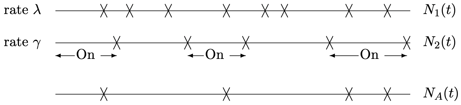
Let \(\left\{N_{A}(t) ; t \geq 0\right\}\) be the switched process; that is \(N_{A}(t)\) includes the arrivals from \(\{N_{1}(t) ; t> 0\}\) during periods when \(N_{2}(t)\) is even and excludes the arrivals from \(\left\{N_{1}(t) ; t>0\right\}\) while \(N_{2}(t)\) is odd.

1. Find the PMF for the number of arrivals of the first process, \(\left\{N_{1}(t) ; t>0\right\}\), during the \(n\)th period when the switch is on.
2. Given that the first arrival for the second process occurs at epoch \(\tau\), find the conditional PMF for the number of arrivals of the first process up to \(\tau\).
3. Given that the number of arrivals of the first process, up to the first arrival for the second process, is \(n\), find the density for the epoch of the first arrival from the second process.
4. Find the density of the interarrival time for \(\left\{N_{A}(t) ; t \geq 0\right\}\). Note: This part is quite messy and is done most easily via Laplace transforms.

Answer

Exercise 2.24

Let us model the chess tournament between Fisher and Spassky as a stochastic process. Let \(X_{i}\), for \(i \geq 1\), be the duration of the ith game and assume that \(\left\{X_{i} ; i \geq 1\right\}\) is a set of IID exponentially distributed rv’s each with density \(\mathrm{f}_{X}(x)=\lambda e^{-\lambda x}\). Suppose that each game (independently of all other games, and independently of the length of the games) is won by Fisher with probability \(p\), by Spassky with probability \(q\), and is a draw with probability \(1-p-q\). The first player to win n games is defined to be the winner, but we consider the match up to the point of winning as being embedded in an unending sequence of games.

1. Find the distribution of time, from the beginning of the match, until the completion of the first game that is won (i.e., that is not a draw). Characterize the process of the number \(\{N(t) ; t>0\}\) of games won up to and including time \(t\). Characterize the process of the number \(\left\{N_{F}(t) ; t \geq 0\right\}\) of games won by Fisher and the number \(\left\{N_{S}(t) ; t \geq 0\right\}\) won by Spassky.
2. For the remainder of the problem, assume that the probability of a draw is zero; i.e., that \(p+q=1\). How many of the first \(2 n-1\) games must be won by Fisher in order to win the match?
3. What is the probability that Fisher wins the match? Your answer should not involve any integrals. Hint: consider the unending sequence of games and use part b).
4. Let \(T\) be the epoch at which the match is completed (i.e., either Fisher or Spassky wins). Find the distribution function of \(T\).
5. Find the probability that Fisher wins and that \(T\) lies in the interval \((t, t+\delta)\) for arbitrarily small \(\delta\).

Answer

Exercise 2.25

1. Find the conditional density of \(S_{i+1}\), conditional on \(N(t)=n\) and \(S_{i}=s_{i}\).
2. Use part a) to find the joint density of \(S_{1}, \ldots, S_{n}\) conditional on \(N(t)=n\). Verify that your answer agrees with (2.37).

Answer

Exercise 2.26

A two-dimensional Poisson process is a process of randomly occurring special points in the plane such that \ref{i} for any region of area \(A\) the number of special points in that region has a Poisson distribution with mean \(\lambda A\), and (ii) the number of special points in nonoverlapping regions is independent. For such a process consider an arbitrary location in the plane and let \(X\) denote its distance from its nearest special point (where distance is measured in the usual Euclidean manner). Show that

1. \(\operatorname{Pr}\{X>t\}=\exp \left(-\lambda \pi t^{2}\right)\)
2. \(\mathrm{E}[X]=1 /(2 \sqrt{\lambda})\)

Answer

Exercise 2.27

This problem is intended to show that one can analyze the long term behavior of queueing problems by using just notions of means and variances, but that such analysis is awkward, justifying understanding the strong law of large numbers. Consider an M/G/1 queue. The arrival process is Poisson with \(\lambda=1\). The expected service time, \(\mathrm{E}[Y]\), is 1/2 and the variance of the service time is given to be 1.

1. Consider \(S_{n}\), the time of the nth arrival, for \(n=10^{12}\). With high probability, \(S_{n}\) will lie within 3 standard derivations of its mean. Find and compare this mean and the \(3 \sigma\) range.
2. Let \(V_{n}\) be the total amount of time during which the server is busy with these \(n\) arrivals (i.e., the sum of \(10^{12}\) service times). Find the mean and \(3 \sigma\) range of \(V_{n}\).
3. Find the mean and \(3 \sigma\) range of \(I_{n}\), the total amount of time the server is idle up until \(S_{n}\) (take \(I_{n}\) as \(S_{n}-V_{n}\), thus ignoring any service time after \(S_{n}\)).
4. An idle period starts when the server completes a service and there are no waiting arrivals; it ends on the next arrival. Find the mean and variance of an idle period. Are successive idle periods IID?
5. Combine \ref{c} and \ref{d} to estimate the total number of idle periods up to time \(S_{n}\). Use this to estimate the total number of busy periods.
6. Combine \ref{e} and \ref{b} to estimate the expected length of a busy period.

Answer

Exercise 2.28

The purpose of this problem is to illustrate that for an arrival process with independent but not identically distributed interarrival intervals, \(X_{1}, X_{2}, \ldots\), the number of arrivals \(N(t)\) in the interval \((0, t]\) can be a defective rv. In other words, the ‘counting process’ is not a stochastic process according to our definitions. This illustrates that it is necessary to prove that the counting rv’s for a renewal process are actually rv’s.

1. Let the distribution function of the \(i\)th interarrival interval for an arrival process be \(\mathrm{F}_{X_{i}}\left(x_{i}\right)=1-\exp \left(-\alpha^{i} x_{i}\right)\) for some fixed \(\alpha \in(0,1)\). Let \(S_{n}=X_{1}+\cdots X_{n}\) and show that

   \(\mathrm{E}\left[S_{n}\right]=\frac{1-\alpha^{n-1}}{1-\alpha}\)

2. Sketch a ‘reasonable’ sample path for \(N(t)\).
3. Find \(\sigma_{S_{n}}^{2}\)
4. Use the Chebyshev inequality on \(\operatorname{Pr}\left\{S_{n} \geq t\right\}\) to find an upper bound on \(\operatorname{Pr}\{N(t) \leq n\}\) that is smaller than 1 for all \(n\) and for large enough \(t\). Use this to show that \(N(t)\) is defective for large enough \(t\).

Answer