3.8: Exercises

Exercise 3.1

Let \([P]\) be the transition matrix for a finite state Markov chain and let state \(i\) be recurrent. Prove that \(i\) is aperiodic if \(P_{i i}>0\).

Exercise 3.2

Show that every Markov chain with \( \mathrm{M}<\infty\) states contains at least one recurrent set of states. Explaining each of the following statements is sufficient.

1. If state \(i_{1}\) is transient, then there is some other state \(i_{2}\) such that \(i_{1} \rightarrow i_{2}\) and \(i_{2} \not \rightarrow i_{1}\).
2. If the \(i_{2}\) of part a) is also transient, there is an \(i_{3}\) such that \(i_{2} \rightarrow i_{3}\), \(i_{3} \not \rightarrow i_{2}\), and consequently \(i_{1} \rightarrow i_{3}\), \(i_{3} \not \rightarrow i_{1}\).
3. Continuing inductively, if \(i_{k}\) is also transient, there is an \(i_{k+1}\) such that \(i_{j} \rightarrow i_{k+1}\) and \(i_{k+1} \not \rightarrow i_{j}\) for \(1 \leq j \leq k\).
4. Show that for some \(k \leq \mathbf{M}\), \(k\) is not transient, i.e., it is recurrent, so a recurrent class exists.

Exercise 3.3

Consider a finite-state Markov chain in which some given state, say state 1, is accessible from every other state. Show that the chain has at most one recurrent class \(\mathcal{R}\) of states and state \(1 \in \mathcal{R}\). (Note that, combined with Exercise 3.2, there is exactly one recurrent class and the chain is then a unichain.)

Exercise 3.4

Show how to generalize the graph in Figure 3.4 to an arbitrary number of states \(\mathrm{M} \geq 3\) with one cycle of M nodes and one of M − 1 nodes. For M = 4, let node 1 be the node not in the cycle of M − 1 nodes. List the set of states accessible from node 1 in \(n\) steps for each \(n \leq 12\) and show that the bound in Theorem 3.2.4 is met with equality. Explain why the same result holds for all larger M

Exercise 3.5 (Proof of Theorem 3.2.4)

1. Show that an ergodic Markov chain with M states must contain a cycle with \(\tau<\mathrm{M}\) states. Hint: Use ergodicity to show that the smallest cycle cannot contain M states.
2. Let \(\ell\) be a fixed state on this cycle of length \(\tau\). Let \(\mathcal{T}(m)\) be the set of states accessible from \(\ell\) in \(m\) steps. Show that for each \(m \geq 1\), \(\mathcal{T}(m) \subseteq \mathcal{T}(m+\tau)\). Hint: For any given state \(j \in \mathcal{T}(m)\), show how to construct a walk of \(m+\tau\) steps from \(\ell\) to \(j\) from the assumed walk of \(m\) steps.
3. Define \(\mathcal{T}(0)\) to be the singleton set \(\{i\}\) and show that

   \(\mathcal{T}(0) \subseteq \mathcal{T}(\tau) \subseteq \mathcal{T}(2 \tau) \subseteq \cdots \subseteq \mathcal{T}(n \tau) \subseteq \cdots.\)

4. Show that if one of the inclusions above is satisfied with equality, then all subsequent inclusions are satisifed with equality. Show from this that at most the first \(M −1\) inclusions can be satisfied with strict inequality and that \(\mathcal{T}(n \tau)=\mathcal{T}((M-1) \tau) \text { for all } n \geq M-1\).
5. Show that all states are included in \(\mathcal{T}((M-1) \tau)\).
6. Show that \(P_{i j}^{(\mathrm{M}-1)^{2}+1}>0\) for all \(i, j\).

Exercise 3.6

Consider a Markov chain with one ergodic class of \(m\) states, say \(\{1,2, \ldots, m\}\) and \(\mathrm{M}-m\) other states that are all transient. Show that \(P_{i j}^{n}>0\) for all \(j \leq m\) and \(n \geq(m-1)^{2}+1+\mathrm{M}-m\)

Exercise 3.7

1. Let \(\tau\) be the number of states in the smallest cycle of an arbitrary ergodic Markov chain of \(\mathrm{M} \geq 3\) states. Show that \(P_{i j}^{n}>0\) for all \(n \geq(\mathrm{M}-2) \tau+\mathrm{M}\). Hint: Look at the proof of Theorem 3.2.4 in Exercise 3.5.
2. For \(\tau=1\), draw the graph of an ergodic Markov chain (generalized for arbitrary \(\mathrm{M} \geq 3\)) for which there is an \(i\), \(j\) for which \(P_{i j}^{n}=0\) for \(n=2 \mathrm{M}-3\). Hint: Look at Figure 3.4.
3. For arbitrary \(\tau<\mathrm{M}-1\), draw the graph of an ergodic Markov chain (generalized for arbitrary M) for which there is an \(i\), \(j\) for which \(P_{i j}^{n}=0\) for \(n=(\mathrm{M}-2) \tau+\mathrm{M}-1\).

Exercise 3.8

A transition probability matrix \([P]\) is said to be doubly stochastic if

\(\sum_{j} P_{i j}=1 \quad \text { for all } i ;\quad \sum_{i} P_{i j}=1 \quad \text { for all } j\)

That is, the row sum and the column sum each equal 1. If a doubly stochastic chain has M states and is ergodic (i.e., has a single class of states and is aperiodic), calculate its steady-state probabilities.

Exercise 3.9

1. Find the steady-state probabilities \(\pi_{0}, \ldots, \pi_{k-1}\) for the Markov chain below. Express your answer in terms of the ratio \(\rho=p / q\). Pay particular attention to the special case \(\rho=1\).
2. Sketch \(\pi_{0}, \ldots, \pi_{k-1}\). Give one sketch for \(\rho=1 / 2\), one for \(\rho=1\), and one for \(\rho=2\).
3. Find the limit of \(\pi_{0}\) as \(k\) approaches \(\infty\); give separate answers for \(\rho<1\), \(\rho=1\), and \(\rho>1\). Find limiting values of \(\pi_{k-1}\) for the same cases.

   

Exercise 3.10

1. Find the steady-state probabilities for each of the Markov chains in Figure 3.2. Assume that all clockwise probabilities in the first graph are the same, say \(p\), and assume that \(P_{4,5}=P_{4,1}\) in the second graph.
2. Find the matrices \([P]^{2}\) for the same chains. Draw the graphs for the Markov chains represented by \([P]^{2}\), i.e., the graph of two step transitions for the original chains. Find the steady-state probabilities for these two step chains. Explain why your steady-state probabilities are not unique.
3. Find \(\lim _{n \rightarrow \infty}\left[P^{2 n}\right]\) for each of the chains.

Exercise 3.11

1. Assume that \(\boldsymbol{\nu}^{(i)}\) is a right eigenvector and \(\boldsymbol{\pi}^{(j)}\) is a left eigenvector of an M by M stochastic matrix \([P]\) where \(\lambda_{i} \neq \lambda_{j}\). Show that \(\boldsymbol{\pi}^{(j)} \boldsymbol{\nu}^{(i)}=0\). Hint: Consider two ways of finding \(\boldsymbol{\pi}^{(j)}[P] \boldsymbol{\nu}^{(i)}\).
2. Assume that \([P]\) has M distinct eigenvalues. The right eigenvectors of \([P]\) then span M space (see section 5.2 of Strang, [19]), so the matrix \([U]\) with those eigenvectors as columns is nonsingular. Show that \(U^{-1}\) is a matix whose rows are the M left eigenvectors of \([P]\). Hint: use part a).
3. For each \(i\), let \(\left[\Lambda^{(i)}\right]\) be a diagonal matrix with a single nonzero element, \(\left[\Lambda_{i i}^{(i)}\right]=\lambda_{i}\). Assume that \(\boldsymbol{\pi}_{i} \boldsymbol{\nu}_{k}=0\). Show that

   \(\boldsymbol{\nu}^{(j)}\left[\Lambda^{(i)}\right] \boldsymbol{\pi}^{(k)}=\lambda_{i} \delta_{i k} \delta_{j k},\)

   where \(\delta_{i k}\) is 1 if \(i=k\) and 0 otherwise. Hint visualize straightforward vector/matrix multiplication.

4. Verify (3.30).

Exercise 3.12

1. Let \(\lambda_{k}\) be an eigenvalue of a stochastic matrix \([P]\) and let \(\boldsymbol{\pi}^{(k)}\) be an eigenvector for \(\lambda_{k}\). Show that for each component \(\pi_{j}^{(k)}\) of \(\boldsymbol{\pi}^{(k)}\) and each \(n\) that

   \(\lambda_{k}^{n} \pi_{j}^{(k)}=\sum_{i} \pi_{i}^{(k)} P_{i j}^{n}.\)

2. By taking magnitudes of each side, show that

   \(\left|\lambda_{k}\right|^{n}\left|\pi_{j}^{(k)}\right| \leq \mathrm{M}.\)

3. Show that \(\left|\lambda_{k}\right| \leq 1\).

Exercise 3.13

Consider a finite state Markov chain with matrix \([P]\) which has \(\kappa\) aperiodic recurrent classes, \(\mathcal{R}_{1}, \ldots, \mathcal{R}_{\kappa}\) and a set \(\mathcal{T}\) of transient states. For any given recurrent class \(\ell\), consider a vector \(\boldsymbol{\nu}\) such that \(\nu_{i}=1\) for each \(i \in \mathcal{R}_{\ell}\), \(\nu_{i}=\lim _{n \rightarrow \infty} \operatorname{Pr}\left\{X_{n} \in \mathcal{R}_{\ell} \mid X_{0}=i\right\}\) for each \(i \in \mathcal{T}\), and \(\nu_{i}=0\) otherwise. Show that \(\boldsymbol{\nu}\) is a right eigenvector of \([P]\) with eigenvalue 1. Hint: Redraw Figure 3.5 for multiple recurrent classes and first show that \(\nu\) is an eigenvector of \(\left[P^{n}\right]\) in the limit.

Exercise 3.14

Answer the following questions for the following stochastic matrix \([P]\)

\([P]=\left[\begin{array}{ccc}
1 / 2 & 1 / 2 & 0 \\
0 & 1 / 2 & 1 / 2 \\
0 & 0 & 1
\end{array}\right].\)

1. Find \([P]^{n}\) in closed form for arbitrary \(n>1\).
2. Find all distinct eigenvalues and the multiplicity of each distinct eigenvalue for \([P]\).
3. Find a right eigenvector for each distinct eigenvalue, and show that the eigenvalue of multiplicity 2 does not have 2 linearly independent eigenvectors.
4. Use \ref{c} to show that there is no diagonal matrix \([\Lambda]\) and no invertible matrix \([U]\) for which \([P][U]=[U][\Lambda]\).
5. Rederive the result of part d) using the result of a) rather than c).

Exercise 3.15

1. Let \(\left[J_{i}\right]\) be a 3 by 3 block of a Jordan form, i.e.,

   \(\left[J_{i}\right]=\left[\begin{array}{ccc}
   \lambda_{i} & 1 & 0 \\
   0 & \lambda_{i} & 1 \\
   0 & 0 & \lambda_{i}
   \end{array}\right]\)

   Show that the \(n\)th power of \(\left[J_{i}\right]\) is given by

   \(\left[J_{i}^{n}\right]=\left[\begin{array}{ccc}
   \lambda_{i}^{n} & n \lambda_{1}^{n-1} & \left(\begin{array}{c}
   n \\
   2
   \end{array}\right) \lambda_{i}^{n-1} \\
   0 & \lambda_{i}^{n} & n \lambda_{1}^{n-1} \\
   0 & 0 & \lambda_{i}^{n}
   \end{array}\right]\)

   Hint: Perhaps the easiest way is to calculate \(\left[J_{i}^{2}\right]\) and \(\left[J_{i}^{3}\right]\) and then use iteration.

2. Generalize a) to a \(k\) by \(k\) block of a Jordan form. Note that the \(n\)th power of an entire Jordan form is composed of these blocks along the diagonal of the matrix.
3. Let \([P]\) be a stochastic matrix represented by a Jordan form \([J]\) as \([P]=U^{-1}[J][U]\) and consider \([U][P]\left[U^{-1}\right]=[J]\). Show that any repeated eigenvalue of \([P]\) (i.e., any eigenvalue represented by a Jordan block of 2 by 2 or more) must be strictly less than 1. Hint: Upper bound the elements of \([U]\left[P^{n}\right]\left[U^{-1}\right]\) by taking the magnitude of the elements of \([U]\) and \(\left[U^{-1}\right]\) and upper bounding each element of a stochastic matrix by 1.
4. Let \(\lambda_{s}\) be the eigenvalue of largest magnitude less than 1. Assume that the Jordan blocks for \(\lambda_{s}\) are at most of size \(k\). Show that each ergodic class of \([P]\) converges at least as fast as \(n^{k} \lambda_{s}^{k}\).

Exercise 3.16

1. Let \(\lambda\) be an eigenvalue of a matrix \([A]\), and let \(\nu\) and \(\boldsymbol{\pi}\) be right and left eigenvectors respectively of \(\lambda\), normalized so that \(\boldsymbol{\pi} \boldsymbol{\nu}=1\). Show that

   \([[A]-\lambda \nu \boldsymbol{\pi}]^{2}=\left[A^{2}\right]-\lambda^{2} \boldsymbol{\nu} \boldsymbol{\pi}\)

2. Show that \(\left[\left[A^{n}\right]-\lambda^{n} \boldsymbol{\nu} \boldsymbol{\pi}\right][[A]-\lambda \nu \boldsymbol{\pi}]=\left[A^{n+1}\right]-\lambda^{n+1} \boldsymbol{\nu} \boldsymbol{\pi}\).
3. Use induction to show that \([[A]-\lambda \boldsymbol{\nu} \boldsymbol{\pi}]^{n}=\left[A^{n}\right]-\lambda^{n} \boldsymbol{\nu} \boldsymbol{\pi}\).

Exercise 3.17

Let \([P]\) be the transition matrix for an aperiodic Markov unichain with the states numbered as in Figure 3.5.

1. Show that \(\left[P^{n}\right]\) can be partitioned as

   \(\left[P^{n}\right]=\left[\begin{array}{cc}
   {\left[P_{\mathcal{T}}^{n}\right]} & {\left[P_{x}^{n}\right]} \\
   0 & {\left[P_{\mathcal{R}}^{n}\right]}
   \end{array}\right]\)

   That is, the blocks on the diagonal are simply products of the corresponding blocks of \([P]\), and the upper right block is whatever it turns out to be.

2. Let \(q_{i}\) be the probability that the chain will be in a recurrent state after \(t\) transitions, starting from state i, i.e., \(q_{i}=\sum_{t<j \leq t+r} P_{i j}^{t}\). Show that \(q_{i}>0\) for all transient \(i\).
3. Let \(q\) be the minimum \(q_{i}\) over all transient \(i\) and show that \(P_{i j}^{n t} \leq(1-q)^{n}\) for all transient \(i, j\) (i.e., show that \(\left[P_{\mathcal{T}}\right]^{n}\) approaches the all zero matrix \([0]\) with increasing \(n\)).
4. Let \(\boldsymbol{\pi}=\left(\boldsymbol{\pi}_{\mathcal{T}}, \boldsymbol{\pi}_{\mathcal{R}}\right)\) be a left eigenvector of \([P]\) of eigenvalue 1. Show that \(\pi_{\mathcal{T}}=0\) and show that \(\boldsymbol{\pi}_{\mathcal{R}}\) must be positive and be a left eigenvector of \(\left[P_{\mathcal{R}}\right]\). Thus show that \(\boldsymbol{\pi}\) exists and is unique (within a scale factor).
5. Show that \(\boldsymbol{e}\) is the unique right eigenvector of \([P]\) of eigenvalue 1 (within a scale factor).

Exercise 3.18

Generalize Exercise 3.17 to the case of a Markov chain \([P]\) with \(m\) recurrent classes and one or more transient classes. In particular,

1. Show that \([P]\) has exactly \(\kappa\) linearly independent left eigenvectors, \(\boldsymbol{\pi}^{(1)}, \boldsymbol{\pi}^{(2)}, \ldots, \boldsymbol{\pi}^{(\kappa)}\) of eigenvalue 1, and that the \(m\)th can be taken as a probability vector that is positive on the \(m\)th recurrent class and zero elsewhere.
2. Show that \([P]\) has exactly \(\kappa\) linearly independent right eigenvectors, \(\boldsymbol{\nu}^{(1)}, \boldsymbol{\nu}^{(2)}, \ldots, \boldsymbol{\nu}^{(\kappa)}\) of eigenvalue 1, and that the mth can be taken as a vector with \(\nu_{i}^{(m)}\) equal to the probability that recurrent class \(m\) will ever be entered starting from state \(i\).
3. Show that

   \(\lim _{n \rightarrow \infty}\left[P^{n}\right]=\sum_{m} \boldsymbol{\nu}^{(m)} \boldsymbol{\pi}^{(m)}\).

Exercise 3.19

Suppose a recurrent Markov chain has period \(d\) and let \(\mathcal{S}_{m}, 1 \leq m \leq d\), be the \(m\)th subset in the sense of Theorem 3.2.3. Assume the states are numbered so that the first \(s_{1}\) states are the states of \(\mathcal{S}_{1}\), the next \(s_{2}\) are those of \(\mathcal{S}_{2}\), and so forth. Thus the matrix \([P]\) for the chain has the block form given by

\([P]=\left[\begin{array}{ccccc}
0 & {\left[P_{1}\right]} & \ddots & \ddots & 0 \\
0 & 0 & {\left[P_{2}\right]} & \ddots & \ddots \\
\ddots & \ddots & \ddots & \ddots & \ddots \\
0 & 0 & \ddots & \ddots & {\left[P_{d-1}\right]} \\
{\left[P_{d}\right]} & 0 & \ddots & \ddots & 0
\end{array}\right],\)

where \(\left[P_{m}\right]\) has dimension \(s_{m}\) by \(s_{m+1}\) for \(1 \leq m \leq d\), where \(d+1\) is interpreted as 1 throughout. In what follows it is usually more convenient to express \(\left[P_{m}\right]\) as an M by M matrix \(\left[P_{m}^{\prime}\right]\) whose entries are 0 except for the rows of \(\mathcal{S}_{m}\) and the columns of \(\mathcal{S}_{m+1}\), where the entries are equal to those of \(\left[P_{m}\right]\). In this view, \([P]=\sum_{m=1}^{d}\left[P_{m}^{\prime}\right]\).

1. Show that \(\left[P^{d}\right]\) has the form

   \(\left[P^{d}\right]=\left[\begin{array}{cccc}
   {\left[Q_{1}\right]} & 0 & \ddots & 0 \\
   0 & {\left[Q_{2}\right]} & \ddots & \ddots \\
   0 & 0 & \ddots & {\left[Q_{d}\right]}
   \end{array}\right],\)

   where \(\left[Q_{m}\right]=\left[P_{m}\right]\left[P_{m+1}\right] \ldots\left[P_{d}\right]\left[P_{1}\right] \ldots\left[P_{m-1}\right]\). Expressing \(\left[Q_{m}\right]\) as an M by M matrix \(\left[Q_{m}^{\prime}\right]\) whose entries are 0 except for the rows and columns of \(\mathcal{S}_{m}\) where the entries are equal to those of \(\left[Q_{m}\right]\), this becomes \(\left[P^{d}\right]=\sum_{m=1}^{d} Q_{m}^{\prime}\).

2. Show that \(\left[Q_{m}\right]\) is the matrix of an ergodic Markov chain, so that with the eigenvectors \(\hat{\boldsymbol{\pi}}_{m}, \hat{\boldsymbol{\nu}}_{m}\) as defined in Exercise 3.18, \(\lim _{n \rightarrow \infty}\left[P^{n d}\right]=\sum_{m=1}^{d} \hat{\boldsymbol{\nu}}^{(m)} \hat{\boldsymbol{\pi}}^{(m)}\).
3. Show that \(\hat{\boldsymbol{\pi}}^{(m)}\left[P_{m}^{\prime}\right]=\hat{\boldsymbol{\pi}}^{(m+1)}\). Note that \(\hat{\boldsymbol{\pi}}^{(m)}\) is an M-tuple that is nonzero only on the components of \(\mathcal{S}_{m}\).
4. Let \(\phi=\frac{2 \pi \sqrt{-1}}{d}\) and let \(\boldsymbol{\pi}^{(k)}=\sum_{m=1}^{d} \hat{\boldsymbol{\pi}}^{(m)} e^{m k \phi}\). Show that \(\boldsymbol{\pi}^{(k)}\) is a left eigenvector of \([P]\) of eigenvalue \(e^{-\phi k}\).

Exercise (continuation of Exerciese 3.19)

1. Show that, with the eigenvectors defined in Exercises 3.19,

   \(\lim _{n \rightarrow \infty}\left[P^{n d}\right][P]=\sum_{i=1}^{d} \boldsymbol{\nu}^{(i)} \boldsymbol{\pi}^{(i+1)},\)

   where, as before, \(d+1\) is taken to be 1.

2. Show that, for \(1 \leq j<d\),

   \(\lim _{n \rightarrow \infty}\left[P^{n d}\right]\left[P^{j}\right]=\sum_{i=1}^{d} \boldsymbol{\nu}^{(i)} \boldsymbol{\pi}^{(i+j)}\).

3. Show that

   \(\lim _{n \rightarrow \infty}\left[P^{n d}\right]\left\{I+[P]+\ldots,\left[P^{d-1}\right]\right\}=\left(\sum_{i=1}^{d} \boldsymbol{\nu}^{(i)}\right)\left(\sum_{i=1}^{d} \boldsymbol{\pi}^{(i+j)}\right)\).

4. Show that

   \(\lim _{n \rightarrow \infty} \frac{1}{d}\left(\left[P^{n}\right]+\left[P^{n+1}\right]+\cdots+\left[P^{n+d-1}\right]\right)=e \pi\),

   where \(\boldsymbol{\pi}\) is the steady-state probability vector for \([P]\). Hint: Show that \(\boldsymbol{e}=\sum_{m} \boldsymbol{\nu}^{(m)}\) and \(\boldsymbol{\pi}=(1 / d) \sum_{m} \boldsymbol{\pi}^{(m)}\).

5. Show that the above result is also valid for periodic unichains.

Exercise 3.21

Suppose \(A\) and \(B\) are each ergodic Markov chains with transition probabilities \(\left\{P_{A_{i}, A_{j}}\right\}\) and \(\left\{P_{B_{i}, B_{j}}\right\}\) respectively. Denote the steady-state probabilities of \(A\) and \(B\) by \(\left\{\pi_{A_{i}}\right\}\) and \(\left\{\pi_{B_{i}}\right\}\) respectively. The chains are now connected and modified as shown below. In particular, states \(A_{1}\) and \(B_{1}\) are now connected and the new transition probabilities \(P^{\prime}\) for the combined chain are given by

\(\begin{array}{lll}
P_{A_{1}, B_{1}}^{\prime} & =\varepsilon, \quad P_{A_{1}, A_{j}}^{\prime}=(1-\varepsilon) P_{A_{1}, A_{j}} & \text { for all } A_{j} \\
P_{B_{1}, A_{1}}^{\prime}&=\delta, \quad P_{B_{1}, B_{j}}^{\prime}=(1-\delta) P_{B_{1}, B_{j}} & \text { for all } B_{j}
\end{array}\)

All other transition probabilities remain the same. Think intuitively of \(\varepsilon\) and \(\delta\) as being small, but do not make any approximations in what follows. Give your answers to the following questions as functions of \(\varepsilon, \delta,\left\{\pi_{A_{i}}\right\} \text { and }\left\{\pi_{B_{i}}\right\}\).

1. Assume that \(\epsilon>0, \delta=0\), (i.e., that \(A\) is a set of transient states in the combined chain). Starting in state \(A_{1}\), find the conditional expected time to return to \(A_{1}\) given that the first transition is to some state in chain \(A\).
2. Assume that \(\epsilon>0, \delta=0\). Find \(T_{A, B}\), the expected time to first reach state \(B_{1}\), starting from state \(A_{1}\). Your answer should be a function of \(\epsilon\) and the original steady state probabilities \(\left\{\pi A_{i}\right\}\) in chain \(A\).
3. Assume \(\varepsilon>0, \delta>0\), find \(T_{B, A}\), the expected time to first reach state \(A_{1}\), starting in state \(B_{1}\). Your answer should depend only on \(\delta\) and \(\left\{\pi_{B_{i}}\right\}\).
4. Assume \(\varepsilon>0\) and \(\delta>0\). Find \(P^{\prime}(A)\), the steady-state probability that the combined chain is in one of the states \(\left\{A_{j}\right\}\) of the original chain \(A\).
5. Assume \(\varepsilon>0, \delta=0\). For each state \(A_{j} \neq A_{1}\) in \(A\), find \(v_{A_{j}}\), the expected number of visits to state \(A_{j}\), starting in state \(A_{1}\), before reaching state \(B_{1}\). Your answer should depend only on \(\varepsilon\) and \(\left\{\pi_{A_{i}}\right\}\).
6. Assume \(\varepsilon>0, \delta>0\). For each state \(A_{j}\) in \(A\), find \(\pi_{A_{j}}^{\prime}\), the steady-state probability of being in state \(A_{j}\) in the combined chain. Hint: Be careful in your treatment of state \(A_{1}\).

Exercise 3.22

Example 3.5.1 showed how to find the expected first passage times to a fixed state, say 1, from all other nodes. It is often desirable to include the expected first recurrence time from state 1 to return to state 1. This can be done by splitting state 1 into 2 states, first an initial state with no transitions coming into it but the original transitions going out, and second, a final trapping state with the original transitions coming in.

1. For the chain on the left side of Figure 3.6, draw the graph for the modified chain with 5 states where state 1 has been split into 2 states.
2. Suppose one has found the expected first-passage-times \(v_{j}\) for states \(j=2\) to 4 (or in general from 2 to M). Find an expression for \(v_{1}\), the expected first recurrence time for state 1 in terms of \(v_{2}, v_{3}, \ldots v_{\mathrm{M}}\) and \(P_{12}, \ldots, P_{1 \mathrm{M}}\).

Exercise 3.23

1. Assume throughout that \([P]\) is the transition matrix of a unichain (and thus the eigenvalue 1 has multiplicity 1). Show that a solution to the equation \([P] \boldsymbol{w}-\boldsymbol{w}=\boldsymbol{r}-g\boldsymbol{e}\) exists if and only if \(\boldsymbol{r}-g\boldsymbol{e}\) lies in the column space of \([P-I]\) where \(I\) is the identity matrix.
2. Show that this column space is the set of vectors \(\boldsymbol{x}\) for which \(\boldsymbol{\pi} \boldsymbol{x}=0\). Then show that \(\boldsymbol{r}-g \boldsymbol{e}\) lies in this column space.
3. Show that, with the extra constraint that \(\boldsymbol{\pi} \boldsymbol{w}=0\), the equation \([P] \boldsymbol{w}-\boldsymbol{w}=\boldsymbol{r}-g \boldsymbol{e}\) has a unique solution.

Exercise 3.24

For the Markov chain with rewards in Figure 3.7,

1. Find the solution to (3.5.1) and find the gain \(g\).
2. Modify Figure 3.7 by letting \(P_{12}\) be an arbitrary probability. Find \(g\) and \(\boldsymbol{w}\) again and give an intuitive explanation of why \(P_{12}\) effects \(w_{2}\).

Exercise 3.25 (Proof of Corollary 3.5.1)

1. Show that the gain per stage \(g\) is 0. Hint: Show that \(\boldsymbol{r}\) is zero where the steady-state vector \(\boldsymbol{\pi}\) is nonzero.
2. Let \(\left[P_{\mathcal{R}}\right]\) be the transition matrix for the recurrent states and let \(\boldsymbol{r}_{\mathcal{R}}=0\) be the reward vector and \(\boldsymbol{w}_{\mathcal{R}}\) the relative-gain vector for \(\left[P_{\mathcal{R}}\right]\). Show that \(\boldsymbol{w}_{\mathcal{R}}=0\). Hint: Use Theorem 3.5.1.
3. Show that \(w_{i}=0\) for all \(i \in \mathcal{R}\). Hint: Compare the relative-gain equations for \([P]\) to those for \(\left[P_{\mathcal{R}}\right]\).
4. Show that for each \(n \geq 0,\left[P^{n}\right] \boldsymbol{w}=\left[P^{n+1}\right] \boldsymbol{w}+\left[P^{n}\right] \boldsymbol{r}\). Hint: Start with the relative-gain equation for \([P] \).
5. Show that \(\boldsymbol{w}=\left[P^{n+1}\right] \boldsymbol{w}+\sum_{m=0}^{n}\left[P^{m}\right] \boldsymbol{r}\). Hint: Sum the result in b).
6. Show that \(\lim _{n \rightarrow \infty}\left[P^{n+1}\right] \boldsymbol{w}=0\) and that \(\lim _{n \rightarrow \infty} \sum_{m=0}^{n}\left[P^{m}\right] \boldsymbol{r}\) is finite, non-negative, and has positive components for \(r_{i}>0\). Hint: Use lemma 3.3.3.
7. Demonstrate the final result of the corollary by using the previous results on \(\boldsymbol{r}=\boldsymbol{r}^{\prime}-\boldsymbol{r}^{\prime \prime}\).

Exercise 3.26

Consider the Markov chain below:

1. Suppose the chain is started in state \(i\) and goes through n transitions; let \(v_{i}(n)\) be the expected number of transitions (out of the total of \(n\)) until the chain enters the trapping state, state 1. Find an expression for \(\boldsymbol{v}(n)=\left(v_{1}(n), v_{2}(n), v_{3}(n)\right)^{\top}\) in terms of \(\boldsymbol{v}(n-1)\) (take \(v_{1}(n)=0\) for all \(n\)). (Hint: view the system as a Markov reward system; what is the value of \(\boldsymbol{r}\)?)
2. Solve numerically for \(\lim _{n \rightarrow \infty} \boldsymbol{v}(n)\). Interpret the meaning of the elements \(v_{i}\) in the solution of (3.32).
3. Give a direct argument why \ref{3.32} provides the solution directly to the expected time from each state to enter the trapping state.

Exercise 3.27

1. Show that \ref{3.48} can be rewritten in the more compact form

   \(\boldsymbol{v}^{*}(n, \boldsymbol{u})=\boldsymbol{v}^{*}\left(1, \boldsymbol{v}^{*}(n-1, \boldsymbol{u})\right)\).

2. Explain why it is also true that

   \[\boldsymbol{v}^{*}(2 n, \boldsymbol{u})=\boldsymbol{v}^{*}\left(n, \boldsymbol{v}^{*}(n, \boldsymbol{u})\right).\label{3.65} \]

3. One might guess that \ref{3.65} could be used iteratively, finding \(\boldsymbol{v}^{*}\left(2^{n+1}, \boldsymbol{u}\right)\) from \(\boldsymbol{v}^{*}\left(2^{n}, \boldsymbol{u}\right)\). Explain why this is not possible in any straighttforward way. Hint: Think through explicitly how one might calculate \(\boldsymbol{v}^{*}\left(n, \boldsymbol{v}^{*}(n, \boldsymbol{u})\right)\) from \(\boldsymbol{v}^{*}(n, \boldsymbol{u})\).

Exercise 3.28

Consider a sequence of IID binary rv’s \(X_{1}, X_{2}, \ldots\) Assume that \(\operatorname{Pr}\left\{X_{i}=1\right\}=p_1\), \(\operatorname{Pr}\left\{X_{i}=0\right\}=p_{0}=1-p_{1}\). A binary string \(\left(a_{1}, a_{2}, \ldots, a_{k}\right)\) occurs at time \(n\) if \(X_{n}=a_{k}, X_{n-1}=a_{k-1}, \ldots X_{n-k+1}=a_{1}\). For a given string \(\left(a_{1}, a_{2}, \ldots, a_{k}\right)\), consider a Markov chain with \(k+1\) states \(\{0,1, \ldots, k\}\). State 0 is the initial state, state \(k\) is a final trapping state where \(\left(a_{1}, a_{2}, \ldots, a_{k}\right)\) has already occurred, and each intervening state \(i\), \(0<i<k\), has the property that if the subsequent \(k-i\) variables take on the values \(a_{i+1}, a_{i+2}, \ldots, a_{k}\), the Markov chain will move successively from state \(i\) to \(i+1\) to \(i+2\) and so forth to \(k\). For example, if \(k=2\) and \(\left(a_{1}, a_{2}\right)=(0,1)\), the corresponding chain is given by

1. For the chain above, find the mean first-passage time from state 0 to state 2.
2. For parts b) to d), let \(\left(a_{1}, a_{2}, a_{3}, \ldots, a_{k}\right)=(0,1,1, \ldots, 1)\), i.e., zero followed by \(k-1\) ones. Draw the corresponding Markov chain for \(k = 4\).
3. Let \(v_{i}\), \(1 \leq i \leq k\) be the expected first-passage time from state \(i\) to state \(k\). Note that \(v_{k}=0\). Show that \(v_{0}=1 / p_{0}+v_{1}\).
4. For each \(i\), \(1 \leq i<k\), show that \(v_{i}=\alpha_{i}+v_{i+1}\) and \(v_{0}=\beta_{i}+v_{i+1}\) where \(\alpha_{i}\) and \(\beta_{i}\) are each a product of powers of \(p_{0}\) and \(p_{1}\). Hint: use induction, or iteration, starting with \(i=1\), and establish both equalities together.
5. Let \(k=3\) and let \(\left(a_{1}, a_{2}, a_{3}\right)=(1,0,1)\). Draw the corresponding Markov chain for this string. Evaluate \(v_{0}\), the expected first-passage time for the string 1,0,1 to occur.

Exercise 3.29

1. Find \(\lim _{n \rightarrow \infty}\left[P^{n}\right]\) for the Markov chain below. Hint: Think in terms of the long term transition probabilities. Recall that the edges in the graph for a Markov chain correspond to the positive transition probabilities.
2. Let \(\boldsymbol{\pi}^{(1)}\) and \(\boldsymbol{\pi}^{(2)}\) denote the first two rows of \(\lim _{n \rightarrow \infty}\left[P^{n}\right]\) and let \(\boldsymbol{\nu}^{(1)}\) and \(\boldsymbol{\nu}^{(2)}\) denote the first two columns of \(\lim _{n \rightarrow \infty}\left[P^{n}\right]\). Show that \(\boldsymbol{\pi}^{(1)}\) and \(\boldsymbol{\pi}^{(2)}\) are independent left eigenvectors of \([P]\), and that \(\boldsymbol{\nu}^{(1)}\) and \(\boldsymbol{\nu}^{(2)}\) are independent right eigenvectors of \([P]\). Find the eigenvalue for each eigenvector.

   

3. Let \(\boldsymbol{r}\) be an arbitrary reward vector and consider the equation

   \[\boldsymbol{w}+g^{(1)} \boldsymbol{\nu}^{(1)}+g^{(2)} \boldsymbol{\nu}^{(2)}=\boldsymbol{r}+[P] \boldsymbol{w}\label{3.66} \]

   Determine what values \(g^{(1)}\) and \(g^{(2)}\) must have in order for \ref{3.66} to have a solution. Argue that with the additional constraints \(w_{1}=w_{2}=0\), \ref{3.66} has a unique solution for \(\boldsymbol{w}\) and find that \(\boldsymbol{w}\).

Exercise 3.30

Let \(\boldsymbol{u}\) and \(\boldsymbol{u}^{\prime}\) be arbitrary final reward vectors with \(\boldsymbol{u} \leq \boldsymbol{u}^{\prime}\).

1. Let \(\boldsymbol{k}\) be an arbitrary stationary policy and prove that \(\boldsymbol{v}^{k}(n, \boldsymbol{u}) \leq \boldsymbol{v}^{k}\left(n, \boldsymbol{u}^{\prime}\right)\) for each \(n \geq 1\).
2. For the optimal dynamic policy, prove that \(\boldsymbol{v}^{*}(n, \boldsymbol{u}) \leq \boldsymbol{v}^{*}\left(n, \boldsymbol{u}^{\prime}\right)\) for each \(n \geq 1\). This is known as the monotonicity theorem.
3. Now let \(\boldsymbol{u}\) and \(\boldsymbol{u}^{\prime}\) be arbitrary. Let \(\alpha=\max _{i}\left(u_{i}-u_{i}^{\prime}\right)\). Show that

   \(\boldsymbol{v}^{*}(n, \boldsymbol{u}) \leq \boldsymbol{v}^{*}\left(n, \boldsymbol{u}^{\prime}\right)+\alpha \boldsymbol{e}.\)

Exercise 3.31

Consider a Markov decision problem with M states in which some state, say state 1, is inherently reachable from each other state.

1. Show that there must be some other state, say state 2, and some decision, \(k_{2}\), such that \(P_{21}^{\left(k_{2}\right)}>0\).
2. Show that there must be some other state, say state 3, and some decision, \(k_{3}\), such that either \(P_{31}^{\left(k_{3}\right)}>0\) or \(P_{32}^{\left(k_{3}\right)}>0\).
3. Assume, for some \(i\), and some set of decisions \(k_{2}, \ldots, k_{i}\) that, for each \(j\), \(2 \leq j \leq i\), \(P_{j l}^{\left(k_{j}\right)}>0\) for some \(l<j\) (i.e., that each state from 2 to \(j\) has a non-zero transition to a lower numbered state). Show that there is some state (other than 1 to \(i\)), say \(i+1\) and some decision \(k_{i+1}\) such that \(P_{i+1, l}^{\left(k_{i+1}\right)}>0\) for some \(l \leq i\)l.
4. Use parts a), b), and c) to observe that there is a stationary policy \(\boldsymbol{k}=k_{1}, \ldots, k_{\mathrm{M}}\) for which state 1 is accessible from each other state.

Exercise 3.32

George drives his car to the theater, which is at the end of a one-way street. There are parking places along the side of the street and a parking garage that costs $5 at the theater. Each parking place is independently occupied or unoccupied with probability 1/2. If George parks \(n\) parking places away from the theater, it costs him \(n\) cents (in time and shoe leather) to walk the rest of the way. George is myopic and can only see the parking place he is currently passing. If George has not already parked by the time he reaches the \(n\)th place, he first decides whether or not he will park if the place is unoccupied, and then observes the place and acts according to his decision. George can never go back and must park in the parking garage if he has not parked before.

1. Model the above problem as a 2 state dynamic programming problem. In the “driving” state, state 2, there are two possible decisions: park if the current place is unoccupied or drive on whether or not the current place is unoccupied.
2. Find \(v_{i}^{*}(n, \boldsymbol{u})\), the minimum expected aggregate cost for \(n\) stages (i.e., immediately before observation of the nth parking place) starting in state \(i = 1\) or 2; it is sufficient to express \(v_{i}^{*}(n, \boldsymbol{u})\) in terms of \(v_{i}^{*}(n-1)\). The final costs, in cents, at stage 0 should be \(v_{2}(0)=500, v_{1}(0)=0\).
3. For what values of \(n\) is the optimal decision the decision to drive on?
4. What is the probability that George will park in the garage, assuming that he follows the optimal policy?

Exercise 3.33 (Proof of Corollary 3.6.1)

1. Show that if two stationary policies \(\boldsymbol{k}^{\prime}\) and \(\boldsymbol{k}\) have the same recurrent class \(\mathcal{R}^{\prime}\) and if \(k_{i}^{\prime}=k_{i}\) for all \(i \in \mathcal{R}^{\prime}\), then \(w_{i}^{\prime}=w_{i}\) for all \(i \in \mathcal{R}^{\prime}\). Hint: See the first part of the proof of Lemma 3.6.3.
2. Assume that \(\boldsymbol{k}^{\prime}\) satisfies 3.50 (i.e., that it satisfies the termination condition of the policy improvement algorithm) and that \(\boldsymbol{k}\) satisfies the conditions of part a). Show that \ref{3.64} is satisfied for all states \(\ell\).
3. Show that \(\boldsymbol{w} \leq \boldsymbol{w}^{\prime}\). Hint: Follow the reasoning at the end of the proof of Lemma 3.6.3.

Exercise 3.34

Consider the dynamic programming problem below with two states and two possible policies, denoted \(\boldsymbol{k}\) and \(\boldsymbol{k}^{\prime}\). The policies differ only in state 2.

1. Find the steady-state gain per stage, \(g\) and \(g^{\prime}\), for stationary policies \(\boldsymbol{k}\) and \(\boldsymbol{k}^{\prime}\). Show that \(g=g^{\prime}\).
2. Find the relative-gain vectors, \(\boldsymbol{w}\) and \(\boldsymbol{w}^{\prime}\), for stationary policies \(\boldsymbol{k}\) and \(\boldsymbol{k}^{\prime}\).
3. Suppose the final reward, at stage 0, is \(u_{1}=0\), \(u_{2}=u\). For what range of \(u\) does the dynamic programming algorithm use decision \(\boldsymbol{k}\) in state 2 at stage 1?
4. For what range of \(u\) does the dynamic programming algorithm use decision \(\boldsymbol{k}\) in state 2 at stage 2? at stage \(n\)? You should find that (for this example) the dynamic programming algorithm uses the same decision at each stage \(n\) as it uses in stage 1.
5. Find the optimal gain \(v_{2}^{*}(n, \boldsymbol{u})\) and \(v_{1}^{*}(n, \boldsymbol{u})\) as a function of stage \(n\) assuming \(u=10\).
6. Find \(\lim _{n \rightarrow \infty} v^{*}(n, \boldsymbol{u})\) and show how it depends on \(u\).

Exercise 3.35

Consider a Markov decision problem in which the stationary policies \(\boldsymbol{k}\) and \(\boldsymbol{k}^{\prime}\) each satisfy \ref{3.50} and each correspond to ergodic Markov chains.

1. Show that if \(\boldsymbol{r}^{\boldsymbol{k}^{\prime}}+\left[P^{\boldsymbol{k}^{\prime}}\right] \boldsymbol{w}^{\prime} \geq \boldsymbol{r}^{\boldsymbol{k}}+\left[P^{\boldsymbol{k}}\right] \boldsymbol{w}^{\prime}\) is not satisfied with equality, then \(g^{\prime}>g\).
2. Show that \(\boldsymbol{r}^{\boldsymbol{k}^{\prime}}+\left[P^{\boldsymbol{k}^{\prime}}\right] \boldsymbol{w}^{\prime}=\boldsymbol{r}^{\boldsymbol{k}}+\left[P^{\boldsymbol{k}}\right] \boldsymbol{w}^{\prime}\) (Hint: use part a).
3. Find the relationship between the relative gain vector \(\boldsymbol{w}^{\boldsymbol{k}}\) for policy \(\boldsymbol{k}\) and the relativegain vector \(\boldsymbol{w}^{\prime}\) for policy \(\boldsymbol{k}^{\prime}\). (Hint: Show that \(\boldsymbol{r}^{k}+\left[P^{k}\right] \boldsymbol{w}^{\prime}=g \boldsymbol{e}+\boldsymbol{w}^{\prime}\); what does this say about \(\boldsymbol{w}\) and \(\boldsymbol{w}^{\prime}\)?)
4. Suppose that policy \(\boldsymbol{k}\) uses decision 1 in state 1 and policy \(\boldsymbol{k}^{\prime}\) uses decision 2 in state 1 (i.e., \(k_{1}=1\) for policy \(\boldsymbol{k}\) and \(k_{1}=2\) for policy \(\boldsymbol{k}^{\prime}\)). What is the relationship between \(r_{1}^{(k)}, P_{11}^{(k)}, P_{12}^{(k)}, \ldots P_{1 J}^{(k)}\) for \(k\) equal to 1 and 2?
5. Now suppose that policy \(\boldsymbol{k}\) uses decision 1 in each state and policy \(\boldsymbol{k}^{\prime}\) uses decision 2 in each state. Is it possible that \(r_{i}^{(1)}>r_{i}^{(2)}\) for all \(i\)? Explain carefully
6. Now assume that \(r_{i}^{(1)}\) is the same for all \(i\). Does this change your answer to part f)? Explain.

Exercise 3.36

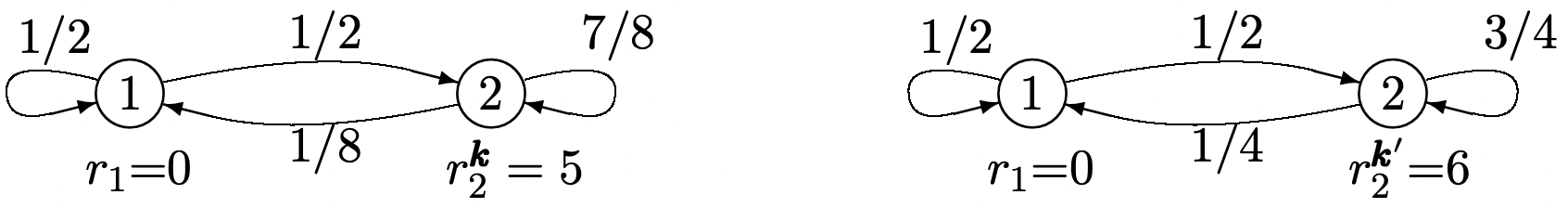
Consider a Markov decision problem with three states. Assume that each stationary policy corresponds to an ergodic Markov chain. It is known that a particular policy \(\boldsymbol{k}^{\prime}=\left(k_{1}, k_{2}, k_{3}\right)=(2,4,1)\) is the unique optimal stationary policy (i.e., the gain per stage in steady state is maximized by always using decision 2 in state 1, decision 4 in state 2, and decision 1 in state 3). As usual, \(r_{i}^{(k)}\) denotes the reward in state \(i\) under decision \(k\), and \(P_{i j}^{(k)}\) denotes the probability of a transition to state \(j\) given state \(i\) and given the use of decision \(k\) in state \(i\). Consider the effect of changing the Markov decision problem in each of the following ways (the changes in each part are to be considered in the absence of the changes in the other parts):

1. \(r_{1}^{(1)}\) is replaced by \(r_{1}^{(1)}-1\).
2. \(r_{1}^{(2)}\) is replaced by \(r_{1}^{(2)}+1\).
3. \(r_{1}^{(k)}\) is replaced by \(r_{1}^{(k)}+1\) for all state 1 decisions \(k\).
4. for all \(i, r_{i}^{\left(k_{i}\right)}\) is replaced by \(r^{\left(k_{i}\right)}+1\) for the decision \(k_{i}\) of policy \(\boldsymbol{k}^{\prime}\).

For each of the above changes, answer the following questions; give explanations:

1. Is the gain per stage, \(g^{\prime}\), increased, decreased, or unchanged by the given change?
2. Is it possible that another policy, \(k \neq k^{\prime}\), is optimal after the given change?

Exercise 3.37

(The Odoni Bound) Let \(\boldsymbol{k}^{\prime}\) be the optimal stationary policy for a Markov decision problem and let \(g^{\prime}\) and \(\boldsymbol{\pi}^{\prime}\) be the corresponding gain and steady-state probability respectively. Let \(v_{i}^{*}(n, \boldsymbol{u})\) be the optimal dynamic expected reward for starting in state \(i\) at stage \(n\) with final reward vector \(\boldsymbol{u}\).

1. Show that \(\min _{i}\left[v_{i}^{*}(n, \boldsymbol{u})-v_{i}^{*}(n-1, \boldsymbol{u})\right] \leq g^{\prime} \leq \max _{i}\left[v_{i}^{*}(n, \boldsymbol{u})-v_{i}^{*}(n-1, \boldsymbol{u})\right]\); \(n \geq 1\). Hint: Consider premultiplying \(\boldsymbol{v}^{*}(n, \boldsymbol{u})-\boldsymbol{v}^{*}(n-1, \boldsymbol{u})\) by \(\boldsymbol{\pi}^{\prime}\) or \(\boldsymbol{\pi}\) where \(\boldsymbol{k}\) is the optimal dynamic policy at stage \(n\).
2. Show that the lower bound is non-decreasing in \(n\) and the upper bound is non-increasing in \(n\) and both converge to \(g^{\prime}\) with increasing \(n\).

Exercise 3.38

Consider an integer-time queueing system with a finite buffer of size 2. At the beginning of the \(n^{\text {th }}\) time interval, the queue contains at most two customers. There is a cost of one unit for each customer in queue (i.e., the cost of delaying that customer). If there is one customer in queue, that customer is served. If there are two customers, an extra server is hired at a cost of 3 units and both customers are served. Thus the total immediate cost for two customers in queue is 5, the cost for one customer is 1, and the cost for 0 customers is 0. At the end of the \(n\)th time interval, either 0, 1, or 2 new customers arrive (each with probability 1/3).

1. Assume that the system starts with \(0 \leq i \leq 2\) customers in queue at time -1 (i.e., in stage 1) and terminates at time 0 (stage 0) with a final cost \(\boldsymbol{u}\) of 5 units for each customer in queue (at the beginning of interval 0). Find the expected aggregate cost \(v_{i}(1, \boldsymbol{u})\) for \(0 \leq i \leq 2\).
2. Assume now that the system starts with \(i\) customers in queue at time -2 with the same final cost at time 0. Find the expected aggregate cost \(v_{i}(2, \boldsymbol{u})\) for \(0 \leq i \leq 2\).
3. For an arbitrary starting time \(−n\), find the expected aggregate cost \(v_{i}(n, \boldsymbol{u})\) for \(0 \leq i \leq 2\).
4. Find the cost per stage and find the relative cost (gain) vector.
5. Now assume that there is a decision maker who can choose whether or not to hire the extra server when there are two customers in queue. If the extra server is not hired, the 3 unit fee is saved, but only one of the customers is served. If there are two arrivals in this case, assume that one is turned away at a cost of 5 units. Find the minimum dynamic aggregate expected cost \(v_{i}^{*}(1), 0 \leq i \leq\), for stage 1 with the same final cost as before.
6. Find the minimum dynamic aggregate expected cost \(v_{i}^{*}(n, \boldsymbol{u})\) for stage \(n\), \(0 \leq i \leq 2\).
7. Now assume a final cost \(\boldsymbol{u}\) of one unit per customer rather than 5, and find the new minimum dynamic aggregate expected cost \(v_{i}^{*}(n, \boldsymbol{u}), 0 \leq i \leq 2\).