7.1: Introduction

Definition 7.1.1. Let \( \{X_i; i ≥ 1 \} \) be a sequence of IID random variables, and let \(S_n = X_1 + X_2 +... + X_n\). The integer-time stochastic process \( \{S_n; n ≥ 1 \} \) is called a random walk, or, more precisely, the one-dimensional random walk based on \( \{ X_i; i ≥ 1\} \).

For any given \(n, \, S_n\) is simply a sum of IID random variables, but here the behavior of the entire random walk process, \( \{ S_n; n ≥ 1\} \), is of interest. Thus, for a given real number \( \alpha > 0\), we might want to find the probability that the sequence \( \{S_n; n ≥ 1\} \) contains any term for which \(S_n ≥ \alpha \) (i.e., that a threshold at \( \alpha \) is crossed) or to find the distribution of the smallest n for which \(S_n ≥ \alpha \).

We know that \(S_n/n\) essentially tends to \( E[X] = \overline{X} \) as \(n \rightarrow \infty \). Thus if \( \overline{X} < 0, \, S_n\) will tend to drift downward and if \(\overline{X} > 0,\, S_n \) will tend to drift upward. This means that the results to be obtained depend critically on whether \( \overline{X} < 0, \, \overline{X} > 0, \text{ or } \overline{X} = 0\). Since results for \( \overline{X} > 0\) can be easily found from results for \(\overline{X} < 0\) by considering {\(−S_n; n ≥ 1\)}, we usually focus on the case \(\overline{X} < 0\).

As one might expect, both the results and the techniques have a very different flavor when \(\overline{X} = 0\), since here \(S_n/n\) essentially tends to 0 and we will see that the random walk typically wanders around in a rather aimless fashion.¹ With increasing \(n, \, \sigma S_n\) increases as \( \sqrt{n} \) (for X both zero-mean and non-zero-mean), and this is often called diffusion.²

The following three subsections discuss three special cases of random walks. The first two, simple random walks and integer random walks, will be useful throughout as examples, since they can be easily visualized and analyzed. The third special case is that of renewal processes, which we have already studied and which will provide additional insight into the general study of random walks.

After this, Sections 7.2 and 7.3 show how two major application areas, G/G/1 queues and hypothesis testing, can be viewed in terms of random walks. These sections also show why questions related to threshold crossings are so important in random walks.

Section 7.4 then develops the theory of threshold crossings for general random walks and Section 7.5 extends and in many ways simplifies these results through the use of stopping rules and a powerful generalization of Wald’s equality known as Wald’s identity.

The remainder of the chapter is devoted to a rather general type of stochastic process called martingales. The topic of martingales is both a subject of interest in its own right and also a tool that provides additional insight Rdensage into random walks, laws of large numbers, and other basic topics in probability and stochastic processes.

Simple random walks

Suppose \(X_1, X_2, . . .\) are IID binary random variables, each taking on the value 1 with probability \(p\) and −1 with probability \(q = 1 − p\). Letting \(S_n = X_1 +...+ X_n\), the sequence of sums {\(S_n; n ≥ 1 \)}, is called a simple random walk. Note that \(S_n\) is the difference between positive and negative occurrences in the first n trials, and thus a simple random walk is little more than a notational variation on a Bernoulli process. For the Bernoulli process, \(X\) takes on the values 1 and 0, whereas for a simple random walk \(X\) takes on the values 1 and -1. For the random walk, if \(X_m = 1\) for \(m\) out of \( n\) trials, then \(S_n = 2m − n\), and

\[ \text{Pr} \{ S_n = 2m-n \} = \dfrac{n!}{m!(n-m)!} p^m (1-p)^{n-m} \nonumber \]

This distribution allows us to answer questions about \(S_n \text{ for any given } n\), but it is not very helpful in answering such questions as the following: for any given integer \( k > 0\), what is the probability that the sequence \(S_1, S_2, . . .\text{ever reaches or exceeds } k\)? This probability can be expressed as³ Pr{\( \bigcup_{n=1}^{\infty} \{ S_n ≥ k \)}} and is referred to as the probability that the random walk crosses a threshold at \(k\). Exercise 7.1 demonstrates the surprisingly simple result that for a simple random walk with \(p ≤ 1/2\), this threshold crossing probability is

\[ \text{Pr} \left\{ \bigcup_{n=1}^{\infty} \{ S_n \geq k \} \right\} = \left( \dfrac{p}{1-p} \right)^k . \nonumber \]

Sections 7.4 and 7.5 treat this same question for general random walks, but the results are far less simple. They also treat questions such as the overshoot given a threshold crossing, the time at which the threshold is crossed given that it is crossed, and the probability of crossing such a positive threshold before crossing any given negative threshold.

Integer-valued random walks

Suppose next that \(X_1, X_2, . . .\) are arbitrary IID integer-valued random variables. We can again ask for the probability that such an integer-valued random walk crosses a threshold at \( k, \, i.e., \) that the event \(\bigcup^{\infty}_{n=1} \{ S_n ≥ k \} \) occurs, but the question is considerably harder than for simple random walks. Since this random walk takes on only integer values, it can be represented as a Markov chain with the set of integers forming the state space. In the Markov chain representation, threshold crossing problems are first passage-time problems. These problems can be attacked by the Markov chain tools we already know, but the special structure of the random walk provides new approaches and simplifications that will be explained in Sections 7.4 and 7.5

Renewal processes as special cases of random walks

If \( X_1, X_2, . . .\) are IID positive random variables, then {\(S_n; n ≥ 1\) } is both a special case of a random walk and also the sequence of arrival epochs of a renewal counting process, {\(N (t); t > 0\) }. In this special case, the sequence {\(S_n; n ≥ 1\) } must eventually cross a threshold at any given positive value \( \alpha \), and the question of whether the threshold is ever crossed becomes uninteresting. However, the trial on which a threshold is crossed and the overshoot when it is crossed are familiar questions from the study of renewal theory. For the renewal counting process, \(N (\alpha ) \) is the largest \( n\) for which \( S_n ≤ \alpha \) and \( N (\alpha ) + 1 \) is the smallest \( n \) for which \( S_n > \alpha , \, i.e., \) the smallest \( n \) for which the threshold at \( \alpha \) is strictly exceeded. Thus the trial at which \( \alpha \) is crossed is a central issue in renewal theory. Also the overshoot, which is \( S_{N (\alpha )+1} − \alpha \) is familiar as the residual life at \(\alpha \).

Figure 7.1 illustrates the difference between general random walks and positive random walks, \(i.e.\), renewal processes. Note that the renewal process in part b) is illustrated with the axes reversed from the conventional renewal process representation. We usually view each renewal epoch as a time (epoch) and view \(N (\alpha )\) as the number of renewals up to time \( \alpha \), whereas with random walks, we usually view the number of trials as a discrete-time variable and view the sum of rv’s as some kind of amplitude or cost. There is no mathematical difference between these viewpoints, and each viewpoint is often helpful.

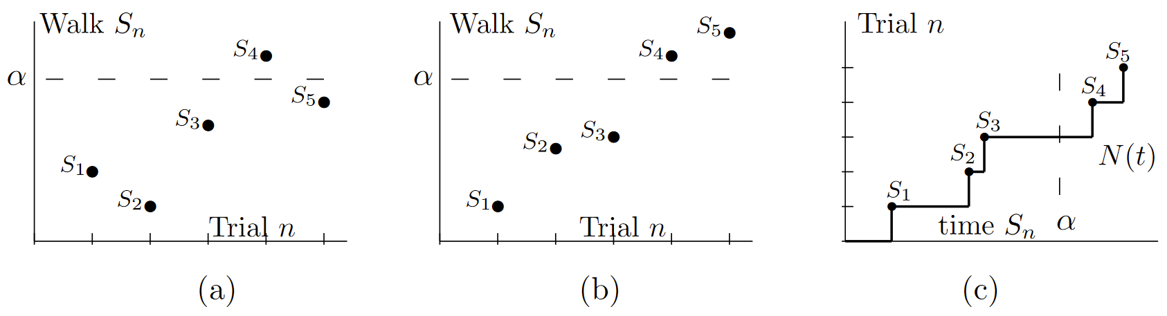
Figure 7.1: The sample function in \ref{a} above illustrates a random walk \( S_1, S_2, . . . ,\) with arbitrary (positive and negative) step sizes {\( X_i; i ≥ 1\) }. The sample function in \ref{b} illustrates a random walk, \( S_1, S_2, . . . ,\) with only positive step sizes {\( X_i > 0; i ≥ 1 \)}. Thus, \(S_1, S_2, . . . ,\) in \ref{b} are sample renewal points in a renewal process. Note that the axes in \ref{b} are reversed from the usual depiction of a renewal process. The usual depiction, illustrated in \ref{c} for the same sample points, also shows the corresponding counting process. The random walks in parts a) and b) each illustrate a threshold at \( \alpha \), which in each case is crossed on trial 4 with an overshoot \( S_4 − \alpha\).

queueing delay in a G/G/1 queue:

Before analyzing random walks in general, we introduce two important problem areas that are often best viewed in terms of random walks. In this section, the queueing delay in a G/G/1 queue is represented as a threshold crossing problem in a random walk. In the next section, the error probability in a standard type of detection problem is represented as a random walk problem.This detection problem will then be generalized to a sequential detection problem based on threshold crossings in a random walk.

Consider a G/G/1 queue with first-come-first-serve (FCFS) service. We shall associate the probability that a customer must wait more than some given time \(\alpha \) in the queue with the probability that a certain random walk crosses a threshold at \(\alpha \). Let \( X_1, X_2, . . .\) be the interarrival times of a G/G/1 queueing system; thus these variables are IID with an arbitrary distribution function \(F_X \ref{x} =\)Pr{\( X_i ≤ x\) }. Assume that arrival 0 enters an empty system at time 0, and thus \( S_n = X_1 +X_2 + ... +X_n\) is the epoch of the \(n^{th}\) arrival after time 0. Let \(Y_0, Y_1, . . . ,\) be the service times of the successive customers. These are independent of {\( X_i; i ≥ 1 \) } and are IID with some given distribution function \( F_Y (y)\). Figure 7.2 shows the arrivals and departures for an illustrative sample path of the process and illustrates the queueing delay for each arrival.

Let \( W_n\) be the queueing delay for the \( n^{th}\) customer, \( n ≥ 1\). The system time for customer \( n\) is then defined as the queueing delay Wn plus the service time \( Y_n\). As illustrated in Figure 7.2, customer \( n ≥ 1\) arrives \( X_n \) time units after the beginning of customer \(n − 1\)’s system time. If \( X_n < W_{n−1} + Y_{n−1}, \, i.e.\), if customer \( n\) arrives before the end of customer \( n − 1\)’s system time, then customer \( n\) must wait in the queue until \( n\) finishes service (in the figure, for example, customer 2 arrives while customer 1 is still in the queue). Thus

\[ W_n = W_{n-1} +Y_{n-1} - X_n \qquad \text{if } X_n \leq W_{n-1} + Y_{n-1} . \nonumber \]

On the other hand, if \( X_n > W_{n−1} + Y_{n−1} \), then customer \(n−1\) (and all earlier customers) have departed when \( n\) arrives. Thus \( n\) starts service immediately and \( W_n = 0\). This is the case for customer 3 in the figure. These two cases can be combined in the single equation

\[ W_n = \text{max} [W_{n-1} + Y_{n-1} - X_n , 0]; \qquad \text{for } n \geq 1; \qquad W_0 = 0 \nonumber \]

______________________________________

1. When \(\overline{X}\) is very close to 0, its behavior for small n resembles that for \(\overline{X} = 0\), but for large enough n the drift becomes significant, and this is reflected in the major results.
2. If we view \(S_n\) as our winnings in a zero-mean game, the fact that \(S_n/n \rightarrow 0\) makes it easy to imagine that a run of bad luck will probably be followed by a run of good luck. However, this is a fallacy here, since the \(X_n\) are assumed to be independent. Adjusting one’s intuition to understand this at a gut level should be one of the reader’s goals in this chapter.
3. This same probability is often expressed as as Pr{\( \text{sup}_{n=1} S_n ≥ k\)}. For a general random walk, the event \(\bigcup_{n \geq 1} \{ S_n ≥ k \} \) is slightly different from \(\text{sup}_{n≥1} S_n ≥ k\), since \(\text{sup}_{n≥1} S_n ≥ k\) can include sample sequences \(s_1, s_2, . . .\) in which a subsequence of values \(s_n \text{ approach } k \text{ as a limit but never quite reach } k\). This is impossible for a simple random walk since all \(s_k\) must be integers. It is possible, but can be shown to have probability zero, for general random walks. It is simpler to avoid this unimportant issue by not using the sup notation to refer to threshold crossings.