7.5: Thresholds, Stopping Rules, and Wald's Identity

The following lemma shows that a random walk with both a positive and negative threshold, say \(\alpha > 0\) and \(\beta < 0\), eventually crosses one of the thresholds. Figure 7.9 illustrates two sample paths and how they cross thresholds. More specifically, the random walk first crosses a threshold at trial \(n\) if \(\beta < S_i < \alpha \) for \(1 \leq i < n\) and either \(S_n \geq \alpha \) or \(S_n \leq \beta \). For now we make no assumptions about the mean or MGF of \(S_n\).

The trial at which a threshold is first crossed is a possibly-defective rv \(J\). The event \(J = n \, (i.e.\), the event that a threshold is first crossed at trial \(n)\), is a function of \(S_1, S_2, . . . , S_n\), and thus, in the notation of Section 4.5, \( J\) is a possibly-defective stopping trial. The following lemma shows that \(J\) is actually a stopping trial, namely that stopping (threshold crossing) eventually happens with probability 1.

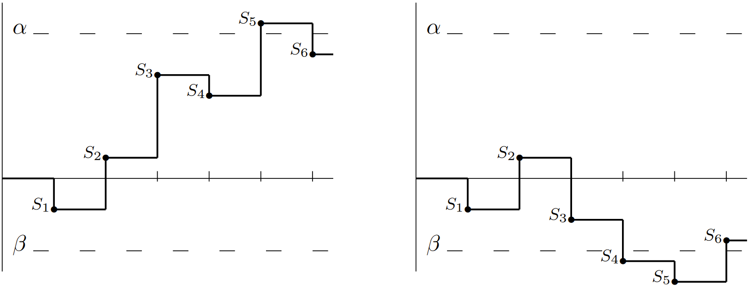
Figure 7.9: Two sample paths of a random walk with two thresholds. In the first, the threshold at \(\alpha \) is crossed at \(J = 5\). In the second, the threshold at \(\beta \) is crossed at \(J = 4\)

Lemma 7.5.1. Let {\(X_i; i \geq 1\)} be IID rv’s, not identically 0. For each \(n \geq 1\), let \(S_n = X_1 +... + X_n\). Let \(\alpha > 0\) and \(\beta < 0\) be arbitrary, and let \( J\) be the smallest \( n\) for which either \(S_n \geq \alpha \) or \( S_n \leq \beta \). Then \( J\) is a random variable (i.e., \( \lim_{m→\infty } \text{Pr}\{ J \geq m \} = 0\) ) and has finite moments of all orders.

Proof: Since \(X\) is not identically 0, there is some \(n\) for which either \(\text{Pr}\{ S_n \leq −\alpha + \beta\} > 0\) or for which \(\text{Pr}\{ S_n \geq \alpha − \beta \} > 0\). For any such \( n\), define \(\epsilon \) by

\[ \epsilon = \max [ \text{Pr} \{ S_n \leq -\alpha + \beta \}, \, \text{Pr}\{ S_n \geq \alpha - \beta \} ] \nonumber \]

For any integer \(k ≥ 1\), given that \(J > n(k − 1)\), and given any value of \( S_{n(k−1)}\) in \((\beta , \alpha )\), a threshold will be crossed by time \(nk\) with probability at least \(\epsilon \). Thus,

\[ \text{Pr} \{ J>nk|J>n(k-1)\} \leq 1-\epsilon \nonumber \]

Iterating on \(k\),

\[ \text{Pr} \{ J>nk \} \leq (1-\epsilon )^k \nonumber \]

This shows that \(J\) is finite with probability 1 and that \(\text{Pr}\{ J ≥ j\}\) goes to 0 at least geomet­rically in \(j\). It follows that the moment generating function \(\mathsf{g}_J (r)\) of \(J\) is finite in a region around \(r = 0\), and that \( J\) has moments of all orders.

\( \square \)

Wald’s identity for two thresholds

Theorem 7.5.1 (Wald’s identity) Let {\(X_i; i ≥ 1\)} be IID and let \(\gamma \ref{r} = \ln \{\mathsf{E} [e^{rX}]\}\) be the semi-invariant MGF of each \(X_i\). Assume \(\gamma (r)\) is finite in the open interval \( (r_−, r_+)\) with \( r_− < 0 < r_+\). For each \( n ≥ 1\), let \( S_n = X_1 +... + X_n\). Let \(\alpha > 0\) and \(\beta < 0\) be arbitrary real numbers, and let \(J\) be the smallest n for which either \( S_n ≥ \alpha \) or \(S_n ≤ \beta \). Then for all \(r ∈ (r_−, r_+)\),

\[ \mathsf{E} [\exp (rS_J-J \gamma (r))] = 1 \nonumber \]

The following proof is a simple application of the tilted probability distributions discussed in the previous section..

Proof: We assume that \(X_i\) is discrete for each \(i\) with the PMF \(\mathsf{p}_X (x)\). For the arbitrary case, the PMF’s must be replaced by distribution functions and the sums by Stieltjes integrals, thus complicating the technical details but not introducing any new ideas.

For any given \( r ∈ (r_−, r_+)\), we use the tilted PMF \(\mathsf{q}_{X,r}(x)\) given in (7.4.4) as

\[ \mathsf{q}_{X,r}(x) = \mathsf{p}_X(x) \exp [r-\gamma \ref{r} ]\nonumber \]

Taking the \( X_i\) to be independent in the tilted probability measure, the tilted PMF for the \(n\)-tuple \(\boldsymbol{X}^n = (X_1, X_2, . . . , X_n)\) is given by

\[ \mathsf{q}_{X^n,r} (\boldsymbol{x}^n) = \mathsf{p}_{\boldsymbol{X}^n}(\boldsymbol{x}^n) \exp [rs_n - n\gamma \ref{r} ] \qquad \text{where } s_n = \sum^n_{i=1}x_i \nonumber \]

Now let \(\mathcal{T}_n\) be the set of \(n\)-tuples \(X_1, . . . , X_n\) such that \(\beta < S_i < \alpha \) for \(1 ≤ i < n\) and either \(S_n ≥ \alpha\) or \(S_n ≤ \beta \). That is, \(\mathcal{T}_n\) is the set of \(\boldsymbol{x}^n\) for which the stopping trial \(J\) has the sample value \(n\). The PMF for the stopping trial \(J\) in the tilted measure is then

\[ \begin{align} \mathsf{q}_{J,r}(n) \quad &= \quad \sum_{\boldsymbol{x}^n\in \mathcal{T}_n} \mathsf{q}_{\boldsymbol{X}^n,r} (\boldsymbol{x}^n) = \sum_{\boldsymbol{x}^n\in \mathcal{T}_n} \mathsf{p}_{\boldsymbol{X}^n} (\boldsymbol{x}^n) \exp [rs_n - n\gamma \ref{r} ] \nonumber \\ &= \quad \mathsf{E} [\exp [rS_n-n\gamma \ref{r} |J=n] \, \text{Pr} \{J = n\} \end{align} \nonumber \]

Lemma 7.5.1 applies to the tilted PMF on this random walk as well as to the original PMF, and thus the sum of \(\mathsf{q}_J (n)\) over \( n\) is 1. Also, the sum over \(n\) of the expression on the right is \(\mathsf{E} [\exp [rS_J − J\gamma (r)]]\), thus completing the proof.

\(\square \)

After understanding the details of this proof, one sees that it is essentially just the statement that \(J\) is a non-defective stopping rule in the tilted probability space.

We next give a number of examples of how Wald’s identity can be used.

relationship of Wald’s identity to Wald’s equality

The trial \( J\) at which a threshold is crossed in Wald’s identity is a stopping trial in the terminology of Chapter 4. If we take the derivative with respect to r of both sides of (7.5.1), we get

\[ \mathsf{E} \left[ [ S_J - J\gamma' \ref{r} \right] \exp \{ rS_J - J\gamma \ref{r} \} = 0 \nonumber \]

Setting \( r = 0\) and recalling that \(\gamma \ref{0} = 0\) and \(\gamma' \ref{0} = \overline{X}\), this becomes Wald’s equality as established in Theorem 4.5.1,

\[ \mathsf{E} [S_J] = \mathsf{E} [J] \overline{X} \nonumber \]

Note that this derivation of Wald’s equality is restricted¹ to a random walk with two thresholds (and this automatically satisfies the constraint in Wald’s equality that \(\mathsf{E} [J] < \infty )\). The result in Chapter 4 is more general, applying to any stopping trial such that \(E [J] < \infty \).

The second derivative of (7.5.1) with respect to \(r\) is

\[ \mathsf{E} [ [ (S_J - J\gamma' (r))^2- J\gamma''(r) ] ] \exp \{rS_J - J\gamma \ref{r} \} = 0 \nonumber \]

At \(r=0\), this is

\[ \mathsf{E} \left[ S^2_J-2JS_J\overline{X} + J^2\overline{X}^2 \right] = \sigma^2_X \mathsf{E} [J] \nonumber \]

This equation is often difficult to use because of the cross term between \( S_J\) and \(J\), but its main application comes in the case where \(\overline{X} = 0\). In this case, Wald’s equality provides no information about \(\mathsf{E}[J]\), but (7.5.4) simplifies to

\[ \mathsf{E} [S^2_J] = \sigma^2_X \mathsf{E} [J] \nonumber \]

Zero-mean simple random walks

As an example of (7.5.5), consider the simple random walk of Section 7.1.1 with \(\text{Pr}\{X=1\} = \text{Pr}\{X= − 1\} = 1/2\), and assume that \(\alpha > 0\) and \(\beta < 0\) are integers. Since \(S_n\) takes on only integer values and changes only by \(\pm 1\), it takes on the value \(\alpha\) or \(\beta \) before exceeding either of these values. Thus \( S_J = \alpha \) or \( S_J = \beta \). Let \(q_{\alpha}\) denote \(\text{Pr}\{S_J = \alpha \}\). The expected value of \(S_J\) is then \(\alpha q_{\alpha} + \beta (1 − q_{\alpha})\). From Wald’s equality, \(\mathsf{E} [S_J ] = 0\), so

\[ q_{\alpha } = \dfrac{-\beta}{\alpha -\beta } ; \qquad 1-q_{\alpha} = \dfrac{\alpha}{\alpha-\beta } \nonumber \]

From (7.5.5),

\[ \sigma^2_X \mathsf{E} [J] = \mathsf{E}[S^2_J] = \alpha^2 q_{\alpha} + \beta^2 (1-q_{\alpha} ) \nonumber \]

Using the value of \(q_{\alpha}\) from (7.5.6) and recognizing that \(\sigma^2_X = 1\),

\[ \mathsf{E} [J] = -\beta \alpha / \sigma^2_X = -\beta \alpha \nonumber \]

As a sanity check, note that if \(\alpha \) and \(\beta \) are each multiplied by some large constant \( k\), then \(\mathsf{E} [J]\) increases by \(k^2\). Since \(\sigma_{S_2}^2 = n\), we would expect \(S_n\) to fluctuate with increasing \( n\), with typical values growing as \(\sqrt{n}\), and thus it is reasonable that the expected time to reach a threshold increases with the product of the distances to the thresholds.

We also notice that if \(\beta \) is decreased toward \(−\infty \), while holding \(\alpha\) constant, then \(q_{\alpha} \rightarrow 1\) and \( \mathsf{E} [J] \rightarrow \infty \). This helps explain Example 4.5.2 where one plays a coin tossing game, stopping when finally ahead. This shows that if the coin tosser has a finite capital \(b, \, i.e.\), stops either on crossing a positive threshold at 1 or a negative threshold at \( −b\), then the coin tosser wins a small amount with high probability and loses a large amount with small probability.

For more general random walks with \(\overline{X} = 0\), there is usually an overshoot when the threshold is crossed. If the magnitudes of \(\alpha \) and \(\beta \) are large relative to the range of \(X\), however, it is often reasonable to ignore the overshoots, and \(-\beta \alpha /\sigma^2_X\) is then often a good approximation to \(\mathsf{E} [J]\). If one wants to include the overshoot, then the effect of the overshoot must be taken into account both in (7.5.6) and (7.5.7).

Exponential bounds on the probability of threshold crossing

We next apply Wald’s identity to complete the analysis of crossing a threshold at \(\alpha > 0\)
when \(\overline{X} < 0\).

Corollary 7.5.1. Under the conditions of Theorem 7.5.1, assume that \(\overline{X} < 0\) and that \(r^* > 0\) exists such that \(\gamma (r^*) = 0\). Then

\[\text{Pr} \{S_J \geq \alpha \}\leq \exp (-r^* \alpha) \nonumber \]

Proof: Wald’s identity, with \(r = r^*\), reduces to \(\mathsf{E} [\exp (r^*S_J )] = 1\). We can express this as

\[\text{Pr} \{S_J \geq \alpha\} \mathsf{E} [\exp (r^*S_J)|S_J\geq \alpha ]+\text{Pr}\{ S_J\leq \beta \} \mathsf{E} [ \exp (r^*S_J)|S_J \leq \beta] = 1 \nonumber \]

Since the second term on the left is nonnegative,

\[ \text{Pr} \{ S_J\geq \alpha \}\mathsf{E}[\exp(r^*S_J)|S_J\geq\alpha] \leq 1 \nonumber \]

Given that \(S_J ≥ \alpha \), we see that \( \exp(r^*S_J ) ≥ \exp(r^*\alpha )\). Thus

\[ \text{Pr}\{ S_J \geq \alpha \} \exp (r^*\alpha)\leq 1 \nonumber \]

which is equivalent to (7.5.9).

This bound is valid for all \( \beta < 0\), and thus is also valid in the limit \(\beta → −\infty \) (see Exercise 7.10 for a more detailed demonstration that (7.5.9) is valid without a lower threshold). We see from this that the case of a single threshold is really a special case of the two threshold problem, but as seen in the zero-mean simple random walk, having a second threshold is often valuable in further understanding the single threshold case. Equation (7.5.9) is also valid for the case of Figure 7.8, where \(\gamma \ref{r} < 0\) for all \(r ∈ (0, r_+]\) and \(r^* = r_+\).

The exponential bound in (7.4.14) shows that \(\text{Pr}\{S_n ≥ \alpha \} ≤ \exp (−r^*\alpha)\) for each \(n\); (7.5.9) is stronger than this. It shows that \(\text{Pr}\{\bigcup_n\{S_n ≥ \alpha\}\} ≤ \exp(−r^*\alpha )\). This also holds in the limit \(\beta → −\infty \).

When Corollary 7.5.1 is applied to the G/G/1 queue in Theorem 7.2.1, (7.5.9) is referred to as the Kingman Bound.

Corollary 7.5.2 (Kingman Bound). Let {\(X_i; i ≥ 1\)} and {\(Y_i; i ≥ 0\)} be the interarrival intervals and service times of a G/G/1 queue that is empty at time 0 when customer 0 arrives. Let {\(U_i = Y_{i−1} − X_i; i ≥ 1\)}, and let \( \gamma \ref{r} = \ln\{\mathsf{E} [e^{U r}]\}\) be the semi-invariant moment generating function of each \(U_i\). Assume that \(\gamma (r)\) has a root at \(r^* > 0\). Then \(W_n\), the queueing delay of the \(n\)th arrival, and \(W\), the steady state queueing delay, satisfy

\[ \text{Pr} \{W_n \geq \alpha \} \leq \text{Pr} \{W\geq\alpha\} \leq \exp (-r^*\alpha ) \quad ; \qquad for \, all \, \alpha>0 \nonumber \]

In most applications, a positive threshold crossing for a random walk with a negative drift corresponds to some exceptional, and often undesirable, circumstance (for example an error in the hypothesis testing problem or an overflow in the G/G/1 queue). Thus an upper bound such as (7.5.9) provides an assurance of a certain level of performance and is often more useful than either an approximation or an exact expression that is very difficult to evaluate. Since these bounds are exponentially tight, they also serve as rough approximations.

For a random walk with \(\overline{X} > 0\), the exceptional circumstance is \(\text{Pr}\{S_J ≤ \beta \}\). This can be analyzed by changing the sign of \( X\) and \(\beta\) and using the results for a negative expected value. These exponential bounds do not work for \(\overline{X} = 0\), and we will not analyze that case here other than the result in (7.5.5).

Note that the simple bound on the probability of crossing the upper threshold in (7.5.9) (and thus also the Kingman bound) is an upper bound (rather than an equality) because, first, the effect of the lower threshold was eliminated (see (7.5.11)), and, second, the overshoot was bounded by 0 (see (7.5.12). The effect of the second threshold can be taken into account by recognizing that \(\text{Pr}\{S_J ≤ \beta \} = 1 − \text{Pr}\{S_J ≥ \alpha \}\). Then (7.5.10) can be solved, getting

\[ \text{Pr}\{S_J \geq \alpha \} = \dfrac{1-\mathsf{E}[\exp (r^*S_J)|S_J \leq \beta ]}{\mathsf{E} [\exp (r^*S_J)|S_J \geq \alpha] - \mathsf{E} [\exp(r^*S_J)|S_J \leq \beta]} \nonumber \]

Solving for the terms on the right side of (7.5.14) usually requires analyzing the overshoot upon crossing a barrier, and this is often difficult. For the case of the simple random walk, overshoots don’t occur, since the random walk changes only in unit steps. Thus, for \(\alpha \) and \(\beta \) integers, we have \(\mathsf{E} [\exp (r^*S_J ) | S_J ≤\beta ] = \exp(r^*\beta )\) and \(\mathsf{E} [\exp (r^*S_J ) | S_J ≥\alpha ] = \exp (r^*\alpha)\). Substituting this in (7.5.14) yields the exact solution

\[ \text{Pr}\{S_J \geq \alpha \} = \dfrac{\exp (-r^* \alpha)[1-\exp (r^*\beta)]}{1-\exp [-r^*(\alpha - \beta )]} \nonumber \]

Solving the equation \(\gamma (r^*) = 0\) for the simple random walk with probabilities \( p\) and \(q\) yields \(r^∗ = \ln (q/p)\). This is also valid if \( X\) takes on the three values −1, 0, and +1 with \(p = \text{ Pr}\{X = 1\}, \, q = \text{Pr}\{X = −1\}\), and \(1 − p − q = \text{Pr}\{X = 0\}\). It can be seen that if \( \alpha \) and \(−\beta \) are large positive integers, then the simple bound of (7.5.9) is almost exact for this example.

Equation (7.5.15) is sometimes used as an approximation for (7.5.14). Unfortunately, for many applications, the overshoots are more significant than the effect of the opposite threshold. Thus (7.5.15) is only negligibly better than (7.5.9) as an approximation, and has the further disadvantage of not being a bound.

If \(\text{Pr} \{S_J ≥ \alpha\}\) must actually be calculated, then the overshoots in (7.5.14) must be taken into account. See Chapter 12 of [8] for a treatment of overshoots.

Binary hypotheses testing with IID observations

The objective of this subsection and the next is to understand how to make binary decisions on the basis of a variable number of observations, choosing to stop observing additional data when a sufficiently good decision can be made. This initial subsection lays the groundwork for this by analyzing the large deviation aspects of binary detection with a large but fixed number of IID observations.

Consider the binary hypothesis testing problem of Section 7.3 in which \( H \) is a binary hy­pothesis with apriori probabilities \(\mathsf{p}_H \ref{0} = p_0\) and \(\mathsf{p}_H \ref{1} = p_1\). The observation \(Y_1, Y_2, . . . ,\) conditional on \(H = 0\), is a sequence of IID rv’s with the probability density \(\mathsf{f}_{Y |H }(y | 0)\). Conditional on \(H = 1\), the observations are IID with density \(\mathsf{f}_{Y |H} (y | 1)\). For any given number \(n\) of sample observations, \(y_1, . . . , y_n\), the likelihood ratio was defined as

\[ \Lambda_n (\boldsymbol{y}) = \prod^n_{i=1} \dfrac{\mathsf{f}_{Y|H} (y_n |0)}{\mathsf{f}_{Y|H} (y_n|1)} \nonumber \]

and the log-likelihood-ratio was defined as

\[ s_n = \sum^n_{i=1} z_n; \qquad \text{where } z_n = \ln \dfrac{\mathsf{f}_{Y|H}(y_n|0)}{\mathsf{f}_{Y|H}(y_n|1)} \nonumber \]

The MAP test gives the maximum aposteriori probability of correct decision based on the n observations \((y_1, . . . , y_n)\). It is defined as the following threshold test:

\[ s_n = \left\{ \begin{array}{cc} >\ln (p_1/p_0) \quad ; \qquad \quad \text{select } \hat{h}=0 \\ \leq \ln (p_1/p_0) \quad ; \qquad \quad \text{select } \hat{h}=1 \end{array} \right. \nonumber \]

We can use the Chernoff bound to get an exponentially tight bound on the probability of error using the the MAP test and given \( H = 1\) (and similarly given \(H = 0\)). That is, \(\text{Pr}\{ e |H = 1\}\) is simply \(\text{Pr}\{S_n ≥ \ln (p_1/p_0) | H=1\}\) where \(S_n\) is the rv whose sample value is given by (7.5.16), \( i.e.,\, S_n = \sum^n_{i=1} Z_n\) where \(Z_n = \ln [f_{Y |H} (Y | 0)/f_{Y |H} (Y | 1)]\). The semi-invariant MGF \(\gamma_1 (r)\) of \(Z\) given \(H = 1\) is

\[ \begin{align} \gamma_1(r) \quad &= \quad \ln\int_y\mathsf{f}_{Y|H}(y|1)\exp \left\{ r \left[ \ln \dfrac{\mathsf{f}_{Y|H}(y|0)}{\mathsf{f}_{Y|H}(y|1)} \right] \right\} dy \nonumber \\ &= \quad \ln \int_y [\mathsf{f}_{Y|H}(y|1)]^{1-r}[\mathsf{f}_{Y|H}(y|0)]^r dy \end{align} \nonumber \]

Surprisingly, we see that \(\gamma_1(1) = \ln\int_y \mathsf{f}_{Y |H} (y | 0) dy = 0\), so that \(r∗ = 1\) for \(\gamma_1(r)\). Since \(\gamma_1(r)\) has a positive second derivative, this shows that \(\gamma_1'(0) < 0\) and \(\gamma_1'(1) > 0\). Figure 7.10 illustrates the optimized exponent in the Chernoff bound,

\[ \text{Pr}\{e|H=1\} \leq \exp \left\{n\left[\min_r\gamma_1(r)-ra \right] \right\} \qquad \text{where } a=\dfrac{1}{n} \ln(p_1/p_0) \nonumber \]

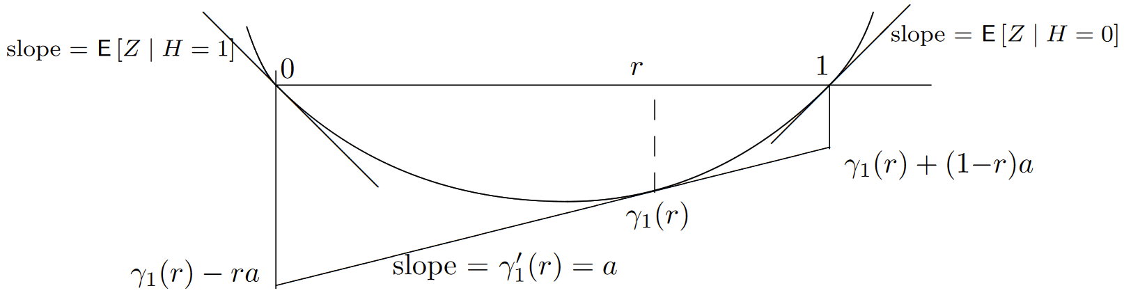
Figure 7.10: Graphical description of the exponents in the optimized Chernoff bounds for \(\text{Pr}\{e | H=1\}≤ \exp \{ n[\gamma_1(r) − ra]\}\) and \(\text{Pr} \{e | H=0\}≤ \exp \{ n[\gamma_1(r) + (1 − r)a]\}\). The slope a is equal to \(\frac{1}{n} \ln(p_1/p_0)\). For an arbitrary threshold test with threshold \(\eta \), the slope \(a\) is \(\frac{1}{n} \ln η\).

We can find the Chernoff bound for \(\text{Pr}\{e | H=0\}\) in the same way. The semi-invariant MGF for \(Z\) conditional on \(H = 0\) is given by

\[ \gamma_0(r) = \ln \int_y [ \mathsf{f}_{Y|H}(y|1)]^{-r}[\mathsf{f}_{Y|H}(y|0)]^{1+r}dy = \gamma_1(r-1) \nonumber \]

We can see from this that the distribution of \(Z\) conditional on \(H = 0\) is the tilted distribution (at \(r = 1\)) of \(Z\) conditional on \(H = 1\). Since \(\gamma_0(r) = \gamma_1(r−1)\), the optimized Chernoff bound for \(\text{Pr}\{e | H=0\}\) is given by

\[ \text{Pr}\{ e|H=0\} \leq \exp \left\{ n \left[ [ \min_r \gamma_1(r)+ (1-r)a \right] \right\} \qquad \text{where } a=\dfrac{1}{n} \ln (p_1/p_0) \nonumber \]

In general, the threshold \(p_1/p_0\) can be replaced by an arbitrary threshold \(η\). As illustrated in Figure 7.10, the slope \(\gamma_1'(r) = \frac{1}{n} \ln(η)\) at which the optimized bound occurs increases with \(η\), varying from \(\gamma'(0) = \mathsf{E} [Z | H=1]\) at \( r = 0\) to \(\gamma'(1) = \mathsf{E} [Z | H=0]\) at \( r = 1\). The tradeoff between the two error exponents are seen to vary as the two ends of an inverted see-saw. One could in principle achieve a still larger magnitude of exponent for \(\text{Pr}\{(\} e | H=1)\) by using \(r > 1\), but this would be somewhat silly since \(\text{Pr}\{e | H=0\}\) would then be very close to 1 and it would usually make more sense to simply decide on \(H = 1\) without looking at the observed data at all.

We can view the tradeoff of exponents above as a large deviation form of the Neyman-Pearson criterion. That is, rather than fixing the allowable value of \(\text{Pr}\{e | H=1\}\) and choosing a test to minimize \(\text{Pr}\{e | H=0\}\), we fix the allowable exponent for \(\text{Pr}\{e | H=1\}\) and then optimize the exponent for \(\text{Pr}\{e | H=1\}\). This is essentially the same as the Neyman-Pearson test, and is a threshold test as before, but it allows us to ignore the exact solution of the Neyman-Pearson problem and focus on the exponentially tight exponents.

Sequential decisions for binary hypotheses

Common sense tells us that it should be valuable to have the ability to make additional observations when the current observations do not lead to a clear choice. With such an ability, we have 3 possible choices at the end of each observation: choose \( \hat{H} = 1\), choose \(\hat{H} =0\), or continue with additional observations. It is evident that we need a stopping time \(J\) to decide when to stop. We assume for the time being that stopping occurs with probability 1, both under hypothesis \(H = 1\) and \(H = 0\), and the indicator rv \(\mathbb{I}_{J=n}\) for each \(n ≥ 1\) is a function of \(Z_1, . . . , Z_n\).

Given \(H = 1\), the sequence of LLR’s {\(S_n; n ≥ 1\)} (where \( S_n =\sum^n_{i=1} Z_i\)) is a random walk. Assume for now that the stopping rule is to stop when the random walk crosses either a threshold² at \(\alpha > 0\) or a threshold at \(β< 0\). Given \(H = 0\), \(S_n = \sum^n_{i=1} Z_n\) is also a random walk (with a different probability measure). The same stopping rule must be used, since the decision to stop at \(n\) can be based only on \(Z_1, . . . , Z_n\) and not on knowledge of \(H\). We saw that the random walk based on \(H = 0\) uses probabilities tilted from those based on \(H = 1\), a fact that is interesting but not necessary here.

We assume that when stopping occurs, the decision \(\hat{h} = 0\) is made if \( S_J ≥ α\) and \(\hat{h} = 1\) is made if \(S_J ≤ β\). Given that \( H = 1\), an error is then made if \(S_J ≥ α\). Thus, using the probability distribution for \(H = 1\), we apply (7.5.9), along with \(r^∗ = 1\), to get

\[ \text{Pr}\{ e|H=1\} \, = \, \text{Pr}\{ S_J \geq \alpha |H=1\} \, \leq \, \exp-\alpha \nonumber \]

Similarly, conditional on \(H = 0\), an error is made if the threshold at \(β\) is crossed before that at \(α\) and the error probability is

\[\text{Pr} \{e|H=0\} \, = \, \text{Pr} \{S_J \leq \beta |H=0 \} \, \leq \, \exp \beta \nonumber \]

The error probabilities can be made as small as desired by increasing the magnitudes of \(α\) and \(β\), but the cost of increasing \(α\) is to increase the number of observations required when \(H = 0\). From Wald’s equality,

\[ \mathsf{E} [J|H=0] \, = \, \dfrac{\mathsf{E}[S_J|H=0]}{\mathsf{E}[Z|H=0]} \,\approx\, \dfrac{\alpha+\mathsf{E}[\text{overshoot}]}{\mathsf{E}[Z|H=0]} \nonumber \]

In the approximation, we have ignored the possibility of \(S_J\) crossing the threshold at \(β\) conditional on \(H = 0\) since this is a very small-probability event when \(α\) and \(β\) have large magnitudes. Thus we see that the expected number of observations (given \(H = 0\)) is essentially linear in \(α\).

We next ask what has been gained quantitatively by using the sequential decision procedure here. Suppose we use a fixed-length test with \(n = α/\mathsf{E} [Z | H=0]\). Referring to Figure 7.10, we see that if we choose the slope \(a = \gamma'(1)\), then the (exponentially tight) Chernoff bound on \(\text{Pr}\{e | H=1\}\) is given by \(e^{−α}\), but the exponent on \(\text{Pr}\{e | H=0\}\) is 0. In other words, by using a sequential test as described here, we simultaneously get the error exponent for \(H = 1\) that a fixed test would provide if we gave up entirely on an error exponent for \(H = 0\), and vice versa.³

A final question to be asked is whether any substantial improvement on this sequential decision procedure would result from letting the thresholds at \(α\) and \(β\) vary with the num­ber of observations. Assuming that we are concerned only with the expected number of observations, the answer is no. We will not carry this argument out here, but it consists of using the Chernoff bound as a function of the number of observations. This shows that there is a typical number of observations at which most errors occur, and changes in the thresholds elsewhere can increase the error probability, but not substantially decrease it.

Joint distribution of crossing time and barrier

Next we look at \(\text{Pr}\{J ≥ n, \, S_J ≥ α\}\), where again we assume that \(\overline{X} < 0\) and that \(\gamma (^r∗) = 0\) for some \(r^∗ > 0\). For any \(r\) in the region where \(\gamma \ref{r} ≤ 0 \, (i.e., \, 0 ≤ r ≤ r^∗)\), we have \(−J\gamma \ref{r} ≥−n\gamma (r)\) for \(J ≥ n\). Thus, from the Wald identity, we have

\[ \begin{align} &1 \geq \mathsf{E}[\exp [rS_J-J\gamma(r)]|J \geq n, \, S_J \geq \alpha ] \text{ Pr}\{ J \geq n, \, S_J \geq \alpha \} \\ &\qquad \geq\exp[r\alpha-n\gamma (r)] \text{Pr}\{J \geq n, \, S_J \geq \alpha \} \nonumber \\ &\text{Pr}\{ J \geq n, \, S_J \geq \alpha \} \leq \exp [-r\alpha+n\gamma (r)]; \qquad \text{for } r\in [0,r^*] \end{align} \nonumber \]

Since this is vaid for all \(r ∈ (0, r^∗]\), we can obtain the tightest bound of this form by minimizing the right hand side of (7.5.21). This is the same minimization (except for the constraint \(r ≤ r^∗\)) as in Figures 7.7. Assume that \(r^∗ < r_+\) (\(i.e.\), that the exceptional situation⁴ of Figure 7.8) does not occur. Define \(n^∗\) as \(α/\gamma'(r^∗)\). The result is then

\[ \text{Pr} \{ J \geq n, S_J \geq \alpha \} \leq \left\{ \begin{array} \exp \exp [n\gamma (r_o) -r_o\alpha] \qquad \text{for } n>n^*, \, \alpha/n = \gamma' (r_o) \\ \\ \exp [-r^*\alpha ] \qquad \qquad n \leq n^* \end{array} \right. \nonumber \]

The interpretation of (7.5.22) is that \(n^∗\) is an estimate of the typical value of \(J\) given that the threshold at \(α\) is crossed. For \(n\) greater than this typical value, (7.5.22) provides a tighter bound on \(\text{Pr}\{J ≥ n, S_J ≥ α\}\) than the bound on \(\text{Pr}\{S_J ≥ α\}\) in (7.5.9), whereas (7.5.22) provides nothing new for \(n ≤ n^∗\). In Section 7.8, we shall derive the slightly stronger result that \(\text{Pr}\left\{ \bigcup_{i\geq n} [S_i ≥ α] \right\}\) is also upper bounded by the right hand side of (7.5.22).

An almost identical upper bound to \(\text{Pr}\{J ≤ n,\, S_J ≥ α\}\) can be found (again assuming that \(r^∗ < r_+\)) by using the Wald identity for \(r > r^∗\). Here \(\gamma \ref{r} > 0\), so \(−J\gamma \ref{r} ≥−n\gamma (r)\) for \(J ≤ n\). The result is

\[ \text{Pr}\{J \leq n, S_J \geq \alpha \} \leq \left\{ \begin{array} \exp \exp[n\gamma (r_o)-r_o\alpha ] \quad \text{for } n<n^*, \, \alpha /n=\gamma' (r_o) \\ \quad \\ \exp [-r^*\alpha] \qquad \qquad n \geq n^* \end{array} \right. \nonumber \]

This strengthens the interpretation of \(n^∗\) as the typical value of \(J\) conditional on crossing the threshold at \(α\). That is, (7.5.23) provides information on the lower tail of the distribution of \(J\) (conditional on \(S_J ≥ α\)), whereas (7.5.22) provides information on the upper tail.

___________________________________

1. This restriction is quite artificial and made simply to postpone any consideration of generalizations until discussing martingales.
2. It is unfortunate that the word ‘threshold’ has a universally accepted meaning for random walks (\(i.e.\), the meaning we are using here), and the word ‘threshold test’ has a universally accepted meaning for hypothesis testing. Stopping when \(S_n\) crosses either \(α\) or \(β\) can be viewed as an extension of an hypothesis testing threshold test in the sense that both the stopping trial and the decision is based only on the LLR, and is based on the LLR crossing either a positive or negative threshold, but the results about threshold tests in Section 7.3 are not necessarily valid for this extension.
3. In the communication context, decision rules are used to detect sequentially transmitted data. The use of a sequential decision rule usually requires feedback from receiver to transmitter, and also requires a variable rate of transmission. Thus the substantial reductions in error probability are accompanied by substantial system complexity.
4. The exceptional situation where \(\gamma (r)\) is negative for \(r ≤ r_+\) and discontinuous at \(r^∗ = r_+ ,\, i.e.\), the situation in Figure 7.8, will be treated in the exercises, and is quite different from the case here. In particular, as can be seen from the figure, the optimized Chernoff bound on \(\text{Pr}\{ S_n ≥ α\}\) is optimized at \(n = 1\).