
7.4: Threshold Crossing Probabilities in Random Walks
- Page ID
- 44635

Let {\(X_i; i \geq 1\)} be a sequence of IID random variables (rv’s ), each with the distribution function \(\mathsf{F}_X (x)\), and let {\(S_n; n \geq 1\)} be a random walk with \( S_n = X_1 +... + X_n\). Let \(g_X \ref{r} = \mathsf{E} [e^{rX} ]\) be the MGF of \( X\) and let \(r_-\) and \( r_+\) be the upper and lower ends of the interval over which \(g(r)\) is finite. We assume throughout that \(r_− < 0 < r_+\). Each of \(r_−\) and \(r_+\) might be contained in the interval where \(g_X (r)\) is finite, and each of \( r_-\) and \(r_+\) might be infinite.
The major objective of this section is to develop results about the probability that the sequence {\(S_n; n \geq 1\)} ever crosses a given threshold \(\alpha > 0, \, i.e., \, \text{Pr}\{ \bigcup^{\infty}_{n=1} \{ S_n \geq α\alpha \}\} \). We assume throughout this section that \(\overline{X} < 0\) and that \(X\) takes on both positive and negative values with positive probability. Under these conditions, we will see that \(\text{Pr}\{\bigcup^{\infty}_{n=1}\{ S_n \geq \alpha \}\}\) is essentially bounded by an exponentially decreasing function of \(\alpha\). In this section and the next, this exponent is evaluated and shown to be exponentially tight with increasing \(\alpha \). The next section also finds an exponentially tight bound on the probability that a threshold at \(\alpha \) is crossed before another threshold at \(\beta < 0\) is crossed.
Chernoff Bound
The Chernoff bound was derived and discussed in Section 1.4.3. It was shown in \ref{1.62} that for any \(r \in (0, r_+)\) and any \( a > \overline{X}\), that
\[ \text{Pr}\{ S_n \geq na\} \leq \exp (n[\gamma_X(r)-ra]) \nonumber \]
where \(\gamma_X \ref{r} = \ln g_X (r)\) is the semi-invariant MGF of X. The tightest bound of this form is given by
\[ \text{Pr}\{ S_n \geq na\} \leq \exp [ n\mu_X(a)] \qquad \text{where } \mu_X(a) = \inf_{r\in (0,r_+)} \gamma_X(r)-ra \nonumber \]
This optimization is illustrated in Figure 7.6 for the case where \(\gamma_X (r)\) is finite for all real \(r\). The optimization is simplified by the fact (shown in Exercise 1.24) that \(\gamma '' \ref{r} > 0\) for \(r \in (0, r_+)\). Lemma 1.4.1 (which is almost obvious from the figure) shows that \(\mu_X \ref{a} < 0\) for \(a > \overline{X}\). This implies that for fixed \(a\), this bound decreases exponentially in \(n\).

| Figure 7.6: Graphical minimization of \(\gamma(r) − ar\). For any \(r, \, \gamma \ref{r} − ar\) is the vertical axis intercept of a line of slope a through the point \( (r, \gamma (r))\). The minimum occurs when the line of slope \(a\) is tangent to the curve, \(i.e.\), for the \( r\) such that \(\gamma '(r) = a\). |
Expressing the optimization in the figure algebraically, we try to minimize \(\gamma \ref{r} − ar\) by setting the derivitive with respect to \(r\) equal to 0. Assuming for the moment that this has a solution and the solution is at some value \(r_o\), we have
\[ \text{Pr}\{ S_n \geq na \} \leq \exp \{ n [\gamma (r_o)-r_o\gamma '(r_o)]\} \qquad \text{where }\gamma '(r_o)=a \nonumber \]
This can be expressed somewhat more compactly by substituting \(\gamma '(r_o)\) for \(a\) in the left side of (7..4.2). Thus, the Chernoff bound says that for each \(r \in (0, r_+)\),
\[ \text{Pr} \{ S_n \geq n\gamma '(r) \} \leq \exp \{ n [ \gamma (r)-r\gamma ' (r)]\} \nonumber \]
In principle, we could now bound the probability of threshold crossing, \(\text{Pr}\{\bigcup^{\infty}_{n=1}\{ S_n \geq \alpha \}\}\), by using the union bound over \(n\) and then bounding each term by (7.4.2). This would be quite tedious and would also give us little insight. Instead, we pause to develop the concept of tilted probabilities. We will use these tilted probabilities in three ways, first to get a better understanding of the Chernoff bound, second to prove that the Chernoff bound is exponentially tight in the limit of large \(n\), and third to prove the Wald identity in the next section. The Wald identity in turn will provide an upper bound on \(\text{Pr}\{ \bigcup^{\infty}_{n=1}\{ S_n \geq \alpha \}\}\) that is essentially exponentially tight in the limit of large \(\alpha \).
Tilted Probabilities
As above, let {\(X_n; n \geq 1\)} be a sequence of IID rv’s and assume that \(g_X (r)\) is finite for \(r \in (r_−, r_+)\). Initially assume that \(X\) is discrete with the PMF \(\mathsf{p}_X (x)\) for each sample value \(x\) of \( X\). For any given \( r \in (r_−, r_+)\), define a new PMF (called a tilted PMF) on \(X\) by
\[ \mathsf{q}_{X,r}(x)=\mathsf{p}_X(x)\exp [rx-\gamma (r)] \nonumber \]
Note that \(\mathsf{q}_{X,r}(x) \geq 0\) for all sample values \(x\) and \(\sum_x \mathsf{ q}_{X,r}(x) = \sum_x \mathsf{ p}_X \ref{x} e^{rx} /\mathsf{E} [e^{rx}] = 1,\) so this is a valid probability assignment
Imagine a random walk, summing IID rv’s \(X_i\), using this new probability assignment rather than the old. We then have the same mapping from sample points of the underlying sample space to sample values of rv’s, but we are dealing with a new probability space, \(i.e.\), we have changed the probability model, and thus we have changed the probabilities in the random walk. We will further define this new probability measure so that the rv’s \(X_1, X_2, . . .\) in this new probability space are IID.1 For every event in the old walk, the same event exists in the new walk, but its probability has changed.
Using (7.4.4), along with the assumption that \(X_1, X_2, . . .\) are independent in the tilted probability assignment, the tilted PMF of an \(n\) tuple \(\boldsymbol{X} = (X_1, X_2, . . . , X_n)\) is given by
\[\mathsf{q}_{\boldsymbol{X}^n,r}(x_1,...,x_n) = \mathsf{p}_{\boldsymbol{X}^n}(x_1,...,x_n) \exp ( \sum_{i=1}^n [rx_i-\gamma (r)] \nonumber \]
Next we must related the PMF of the sum, \(\sum_{i=1}^n X_i\), in the original probability measure to that in the tilted probability measure. From (7.4.5), note that for every \(n\)-tuple \((x_1, . . . , x_n)\) for which \(\sum^n_{i=1} x_i = s_n\) (for any given \( s_n\)) we have
\[ \mathsf{q}_{\boldsymbol{X}^n,r}(x_1,...,x_n) = \mathsf{p}_{\boldsymbol{X}^n}(x_1,...,x_n) \exp [rs_n -n\gamma (r)]\nonumber \]
Summing over all \( \boldsymbol{x}^n\) for which \(\sum^n_{i=1} x_i = s_n\), we then get a remarkable relation between the PMF for \( S_n\) in the original and the tilted probability measures:
\[ \mathsf{q}_{\boldsymbol{S}_n,r}(s_n) = \mathsf{p}_{S_n}(s_n)\exp [rs_n-n\gamma (r)] \nonumber \]
This equation is the key to large deviation theory applied to sums of IID rv’s . The tilted measure of \( S_n\), for positive \( r\), increases the probability of large values of \(S_n\) and decreases that of small values. Since \(S_n\) is an IID sum under the tilted measure, however, we can use the laws of large numbers and the CLT around the tilted mean to get good estimates and bounds on the behavior of \(S_n\) far from the mean for the original measure.
We now denote the mean of \( X\) in the tilted measure as \(\mathsf{E}_r[X]\). Using (7.4.4),
\[ \begin{align} \mathsf{E}_r[X] \quad &= \quad \sum_x x\mathsf{q}_{X,r}(x) = \sum_x \mathsf{p}_X(x) \exp [rx-\gamma \ref{r} ] \nonumber \\ &= \quad \dfrac{1}{g_X(r)} \sum_x \dfrac {d}{dr} \mathsf{p}_X(x) \exp [rx] \nonumber \\ &= \quad \dfrac{g'_X(r)}{g_X(r)} = \gamma' \ref{r} \end{align} \nonumber \]
Higher moments of \(X\) under the tilted measure can be calculated in the same way, but, more elegantly, the MGF of \( X\) under the tilted measure can be seen to be \(\mathsf{E}_r[\exp (tX)] = g_X (t + r)/g_X (r)\).
The following theorem uses (7.4.6) and (7.4.7) to show that the Chernoff bound is exponentially tight.
Theorem 7.4.1. Let {\(X_n; n \geq 1\)} be a discrete IID sequence with a finite MGF for \(r \in (r_−, r_+)\) where \( r_− < 0 < r_+\). Let \( S_n = \sum^n_{i=1}x_i\) for each \(n ≥ 1\). Then for any \( r \in (0, r_+)\), and any \( \epsilon > 0\) and \(\delta > 0\) there is an m such that for all \(n ≥ m\),
\[ \text{Pr}\{S_n \geq n(\gamma' \ref{r} - \in) \} \quad \geq \quad (1-\delta) \exp [n(\gamma (r)-r\gamma' \ref{r} - r\epsilon )] \nonumber \]
Proof: The weak law of large numbers, in the form of (1.76), applies to the tilted measure on each \( S_n\). Writing out the limit on \( n\) there, we see that for any \(\epsilon , \delta \), there is an \( m\) such that for all \(n \geq m\),
\[ \begin{align} 1-\delta \quad &\leq \sum_{(\gamma'(r)-\epsilon )n \leq s_n \leq (\gamma' (r)+\epsilon )n} \mathsf{q}_{S_n,r} (s_n) \nonumber \\ &= \sum_{(\gamma'(r)-\epsilon )n \leq s_n \leq (\gamma' (r)+\epsilon )n} \mathsf{p}_{S_n}(s_n)\exp [rs_n - n \gamma \ref{r} ] \\ &\leq \sum_{(\gamma'(r)-\epsilon )n \leq s_n \leq (\gamma' (r)+\epsilon )n} \mathsf{p}_{S_n}(s_n)\exp [n(r\gamma' \ref{r} +r\epsilon - \gamma (r))] \\ &\leq \sum_{(\gamma' (r)-\epsilon )n \leq s_n} \mathsf{p}_{S_n}(s_n)\exp [ n(r\gamma' \ref{r} + r\epsilon - \gamma (r))] \\ &= \exp [n(r\gamma' \ref{r} + r\epsilon - \gamma (r))] \text{Pr} \{ S_n \geq n (\gamma' \ref{r} - \epsilon ) \} \end{align} \nonumber \]
The equality (7.4.9) follows from (7.4.6) and the inequality (7.4.10) follows because \(s_n \leq \gamma' \ref{r} + \epsilon \) in the sum. The next inequality is the result of adding additional positive terms into the sum, and (7.4.12) simply replaces the sum over a PMF with the probability of the given event. Since (7.4.12) is equivalent to (7.4.8), the proof is complete.
\( \square \)
The structure of the above proof can be used in many situations. A tilted probability measure is used to focus on the tail of a distribution, and then some known result about the tilted distribution is used to derive the desired result about the given distribution.
Back to threshold crossings
The Chernoff bound is convenient (and exponentially tight) for understanding \(\text{Pr}\{ S_n \geq na\} \) as a function of \(n\) for fixed \(a\). It does not give us as much direct insight into \(\text{Pr}\{ S_n \geq α \}\) as a function of \(n\) for fixed \(\alpha \), which tells us something about when a threshold at \(\alpha \) is most likely to be crossed. Additional insight can be achieved by substituing \( \alpha /\gamma' (r_0)\) for \(n\) in (7.4.2), getting
\[ \text{Pr} \{S_n \geq \alpha \} \leq \exp \left\{ \alpha \left[ \dfrac{\gamma (r_o)}{\gamma' (r_o) } -r_o \right] \right\} \qquad \text{where } \gamma' (r_o) = \alpha /n \nonumber \]
A nice graphic interpretation of this equation is given in Figure 7.7. Note that the exponent in \(\alpha \), namely \(\gamma (r_0)/ \gamma' (r_0) − r_0\) is the negative of the horizontal axis intercept of the line of slope \(\gamma' (r_0) = \alpha /n\) in Figure 7.7.
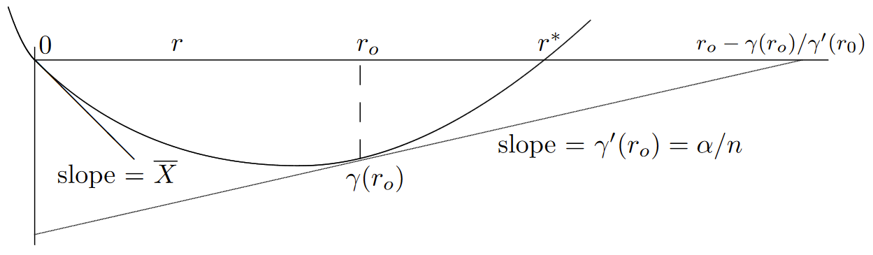
| Figure 7.7: The exponent in \(\alpha \) for \(\text{Pr}\{ S_n \geq \alpha \}\), minimized over r. The minimization is the same as that in Figure 7.6, but \(\gamma (r_o)/ \gamma' (r_o) − r_o\) is the negative of the horizontal axis intercept of the line tangent to \(\gamma (r)\) at \(r = r_0\) |
For fixed \(\alpha \), then, we see that for very large \(n\), the slope \(\alpha /n\) is very small and this horizontal intercept is very large. As \(n\) is decreased, the slope increases, \(r_0\) increases, and the horizontal intercept decreases. When \( r_0\) increases to the point labeled \( r^*\) in the figure, namely the \(r > 0\) at which \(\gamma \ref{r} = 0\), then the exponent decreases to \(r^*\). When \(n\) decreases even further, \(r_0\) becomes larger than \(r^*\) and the horizontal intercept starts to increase again.
Since \(r^∗\) is the minimum horizontal axis intercept of this class of straight lines, we see that the following bound holds for all \( n\),
\[ \text{Pr} \{ S_n \geq \alpha \} \leq \exp (-r^* \alpha ) \qquad \text{for arbitrary } \alpha > 0,n\geq 1 \nonumber \]
where \(r^*\) is the positive root of \(\gamma \ref{r} = 0\).
The graphical argument above assumed that there is some \(r^* > 0\) such that \(\gamma_X (r^*) = 0\). However, if \( r_+ = \infty \), then (since \(X\) takes on positive values with positive probability by assumption) \(\gamma (r)\) can be seen to approach \(\infty \) as \(r \rightarrow \infty\). Thus \(r^*\) must exist because of the continuity of \(\gamma (r)\) in \((r_−, r_+)\). This is summarized in the following lemma.
Lemma 7.4.1. Let {\( S_n = X_1 + ...+ X_n; n \geq 1\)} be a random walk where {\(X_i; i \geq 1\)} is an IID sequence where \( g_X (r)\) exists for all \(r \geq 0\), where \(\overline{X} < 0\), and where \(X\) takes on both positive and negative values with positive probability. Then for all integer \(n > 0\) and all \(\alpha > 0\)
\[ \text{Pr}\{ S_n \geq \alpha \} \leq \exp \{ \alpha [\gamma (r_0)n/\alpha -r_0] \} \leq \exp (-r^*\alpha ) \nonumber \]
where \(\gamma' (r_o) = \alpha /n\).
Next we briefly consider the situation where \(r_+ < \infty\). There are two cases to consider, first where \(\gamma (r_+)\) is infinite and second where it is finite. Examples of these cases are given in Exercise 1.22, parts b) and c) respectively. For the case \(\gamma (r_+) = \infty \), Exercise 1.23 shows that \(\gamma (r)\) goes to \(\infty \) as \(r\) increases toward \(r_+\). Thus \(r^*\) must exist in this case 1 by continuity.
The case \(\gamma (r_+) < \infty \) is best explained by Figure 7.8. As explained there, if \(\gamma' \ref{r} = \alpha /n\) for some \( r_0 < r_+\), then (7.4.2) and (7.4.13) hold as before. Alternatively, if \(\alpha /n > \gamma' (r)\) for all \(r < r_+\), then the Chernoff bound is optimized at \( r = r_+\), and we have
\[ \text{Pr} \{S_n \geq \alpha \} \leq \exp \{ n[\gamma (r_+)-r_+\alpha /n] \} = \exp \{ \alpha [\gamma (r_+)n/\alpha -r_+]\} \nonumber \]
If we modify the definition of \(r^*\) to be the supremum of \( r > 0\) such that \(\gamma \ref{r} < 0\), then \(r^* = r_+\) in this case, and (7.4.15) is valid in general with the obvious modification of \(r_o\).
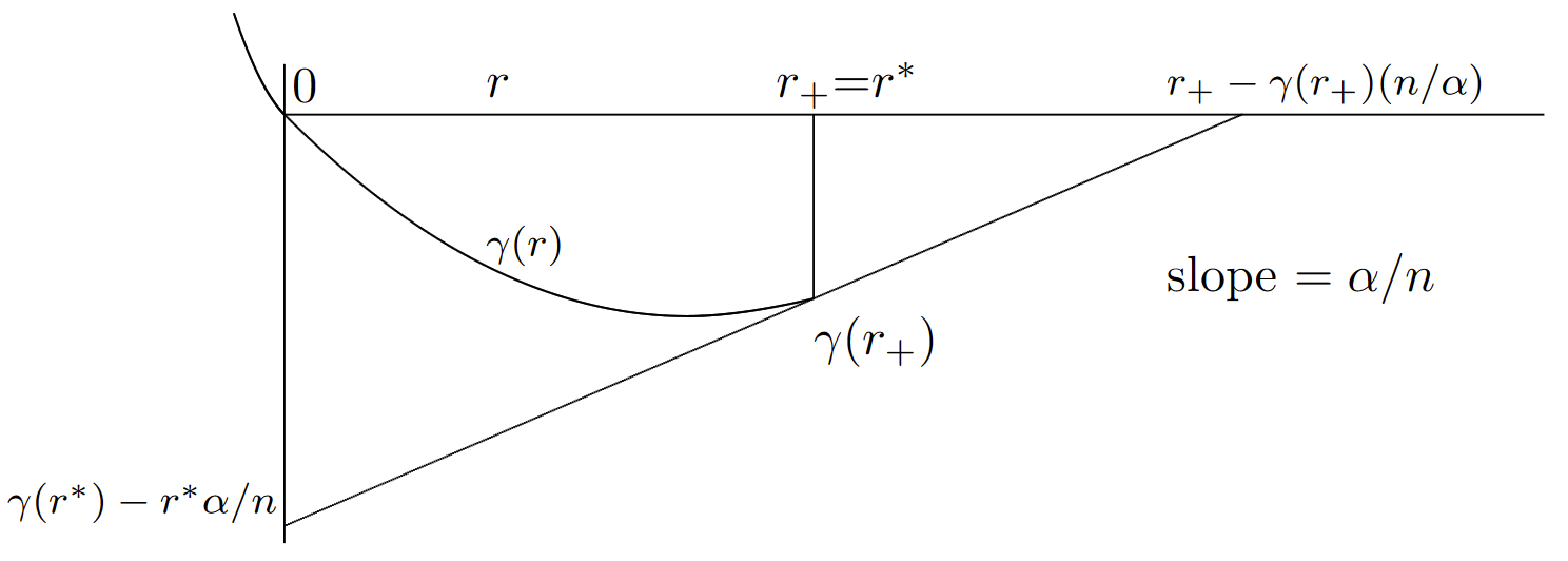
| Figure 7.8: Graphical minimization of \(\gamma \ref{r} − (\alpha /n)r\) for the case where \(\gamma (r^+) < \infty\). As before, for any \(r < r_+\), we can find \(\gamma (r)−r\alpha /n\) by drawing a line of slope \((\alpha /n)\) from the point \((r, \gamma (r))\) to the vertical axis. If \(\gamma' \ref{r} = \alpha /n\) for some \( r < r_+\), the minimum occurs at that \( r\). Otherwise, as shown in the figure, it occurs at \(r = r_+\). |
We could now use this result, plus the union bound, to find an upper bound on the probability of threshold crossing, \(i.e.\), \(\text{Pr}\{\bigcup^{\infty}_{n=1} \{S_n \geq \alpha \}\}\). The coefficients in this are somewhat messy and change according to the special cases discussed above. It is far more instructive and elegant to develop Wald’s identity, which shows that \(\text{Pr}\{ \bigcup_n \{ S_n \geq \alpha \}\} \leq \exp [−\alpha r^*]\). This is slightly stronger than the Chernoff bound approach in that the bound on the probability of the union is the same as that on a single term in the Chernoff bound approach. The main value of the Chernoff bound approach, then, is to provide assurance that the bound is exponentially tight.
______________________________________
- One might ask whether \(X_1, X_2, . . .\) are the same rv’s in this new probability measure as in the old. It is usually convenient to view them as being the same, since they correspond to the same mapping from sample points to sample values in both probability measures. However, since the probability space has changed, one can equally well view them as different rv’s. It doesn’t make any difference which viewpoint is adopted, since all we use the relationship in (7.4.4), and other similar relationships, to calculate probabilities in the original system.