7.3: Detection, Decisions, and Hypothesis Testing

Consider a situation in which we make \(n\) noisy observations of the outcome of a single discrete random variable \(H\) and then guess, on the basis of the observations alone, which sample value of \(H\) occurred. In communication technology, this is called a detection problem. It models, for example, the situation in which a symbol is transmitted over a communication channel and \(n\) noisy observations are received. It similarly models the problem of detecting whether or not a target is present in a radar observation. In control theory, such situations are usually referred to as decision problems, whereas in statistics, they are referred to both as hypothesis testing and statistical inference problems.

The above communication, control, and statistical problems are basically the same, so we discuss all of them using the terminology of hypothesis testing. Thus the sample values of the rv \(H\) are called hypotheses. We assume throughout this section that \(H\) has only two possible values. Situations where \(H\) has more than 2 values can usually be viewed in terms of multiple binary decisions.

It makes no difference in the analysis of binary hypothesis testing what the two hypotheses happen to be called, so we simply denote them as hypothesis 0 and hypothesis 1. Thus \(H\) is a binary rv and we abbreviate its PMF as \(\text{p}_H \ref{0} = p_0 \) and \(\text{p}_H \ref{1} = p_1\). Thus \(p_0\) and \(p_1 = 1 − p_0\) are the a priori probabilities¹ for the two sample values (hypotheses) of the random variable \(H\).

Let \(\boldsymbol{Y} = (Y_1, Y_2, . . . , Y_n)\) be the \(n\) observations. Suppose, for initial simplicity, that these variables, conditional on \(H = 0\) or \(H = 1\), have joint conditional densities, \(f_{\boldsymbol{Y} |H} (\boldsymbol{y} | 0)\) and \(f_{\boldsymbol{Y} |H} (\boldsymbol{y} | 1)\), that are strictly positive over their common region of definition. The case of primary importance in this section (and the case where random walks are useful) is that in which, conditional on a given sample value of \(H\), the rv’s \(Y_1, . . . , Y_n\) are IID. Still assuming for simplicity that the observations have densities, say \(f_{\boldsymbol{Y} |H} (y | \ell) \) for \(\ell = 0\) or \(\ell = 1\), the joint density, conditional on \(H = \ell\), is given by

\[ f_{\boldsymbol{Y}|H}(\boldsymbol{y}|\ell ) = \prod^n_{i=1} f_{Y|H} (y_i|\ell ) \nonumber \]

Note that all components of \(\boldsymbol{Y}\) are conditioned on the same \(H, \, i.e.\), for a single sample value of \( H\), there are \(n\) corresponding sample values of \(Y\).

Assume that it is necessary² to select a sample value for \( H\) on the basis of the sample value \(\boldsymbol{y}\) of the \( n\) observations. It is usually possible for the selection (decision) to be incorrect, so we distinguish the sample value \( h\) of the actual experimental outcome from the sample value \(\hat{h}\) of our selection. That is, the outcome of the experiment specifies \(h\) and \(\boldsymbol{y}\), but only \(\boldsymbol{y}\) is observed. The selection \(\hat{h}\), based only on \(\boldsymbol{y}\), might be unequal to h. We say that an error has occurred if \(\hat{h} \neq h \)

We now analyze both how to make decisions and how to evaluate the resulting probability of error. Given a particular sample of n observations \( \boldsymbol{y} = y_1, y_2, . . . , y_n,\) we can evaluate Pr\(\{ H=0 | \boldsymbol{y}\}\) as

\[ \text{Pr}\{ H=0|\boldsymbol{y} \} = \dfrac{p_0 f_{\boldsymbol{Y}|H} (\boldsymbol{y} | 0)}{p_0f_{\boldsymbol{Y}|H} (\boldsymbol{y}|0)+p_1 f_{\boldsymbol{Y}|H} (\boldsymbol{y}|1)} \nonumber \]

We can evaluate Pr{\(H=1 | \boldsymbol{y}\)} in the same way The ratio of these quantities is given by

\[ \dfrac{ \text{Pr} \{H=0 | \boldsymbol{y} \} }{ \text{Pr} \{H=1 | \boldsymbol{y} \}}= \dfrac{ p_0 f_{\boldsymbol{Y} |H} (\boldsymbol{y} |0)}{p_1 f_{\boldsymbol{Y} |H} (\boldsymbol{y} |1)} \nonumber \]

For a given \(\boldsymbol{y}\), if we select \(\hat{h} = 0\), then an error is made if \(h = 1\). The probability of this event is Pr{\(H = 1 | \boldsymbol{y}\)}. Similarly, if we select \(\hat{h} = 1\), the probability of error is Pr{\(H = 0 | \boldsymbol{y}\)}. Thus the probability of error is minimized, for a given \(\boldsymbol{y}\), by selecting \(\hat{h} =0\) if the ratio in (7.3.3) is greater than 1 and selecting \(\hat{h}=1\) otherwise. If the ratio is equal to 1, the error probability is the same whether \(\hat{h}=0 \) or \(\hat{h}=1\) is selected, so we arbitrarily select \(\hat{h}= 1\) to make the rule deterministic.

The above rule for choosing \(\hat{H}=0\) or \(\hat{H}=1\) is called the Maximum a posteriori probability detection rule, abbreviated as the MAP rule. Since it minimizes the error probability for each \(\boldsymbol{y}\), it also minimizes the overall error probability as an expectation over \(\boldsymbol{Y}\) and \(H\).

The structure of the MAP test becomes clearer if we define the likelihood ratio \( \Lambda (\boldsymbol{y})\) for the binary decision as

\[ \Lambda (\boldsymbol{y}) = \dfrac{f_{\boldsymbol{Y}|H}(\boldsymbol{y}|0)}{f_{\boldsymbol{Y}|H}(\boldsymbol{y}|1)} \nonumber \]

The likelihood ratio is a function only of the observation \(\boldsymbol{y}\) and does not depend on the a priori probabilities. There is a corresponding rv \( \Lambda (\boldsymbol{Y} )\) that is a function³ of \(\boldsymbol{Y}\), but we will tend to deal with the sample values. The MAP test can now be compactly stated as

\[ \Lambda (\boldsymbol{y}) \quad \left\{ \begin{array}{cc} > p_1/p_0 \quad ; & \qquad \text{select }\hat{h}=0 \\ \\ \leq p_1/p_0 \quad ; & \qquad \text{select }\hat{h}=1 \end{array} \right. \nonumber \]

For the primary case of interest, where the n observations are IID conditional on H, the
likelihood ratio is given by

\[ \Lambda (\boldsymbol{y}) = \prod^n_{i=1} \dfrac{f_{Y|H}(y_i|0)}{f_{Y|H}(y_i|1)} \nonumber \]

The MAP test then takes on a more attractive form if we take the logarithm of each side in (7.3.4). The logarithm of \(\Lambda (\boldsymbol{y})\) is then a sum of \(n\) terms, \(\sum^n_{i=1} z_i\), where \(z_i\) is given by

\[ z_i = \ln \dfrac{f_{Y|H}(y_i|0)}{f_{Y|H}(y_i|1)} \nonumber \]

The sample value \(z_i\) is called the log-likelihood ratio of \(y_i\) for each \( i\), and \( \ln \Lambda (\boldsymbol{y})\) is called the log-likelihood ratio of \(\boldsymbol{y}\). The test in (7.3.4) is then expressed as

\[ \sum^n_{i=1} z_i \left\{ \begin{array}{cc} >\ln (p_1/p_0) \quad ; & \qquad \text{select } \hat{h}=0 \\ \\ \leq \ln (p_1/p_0) \quad ; & \qquad \text{select } \hat{h}=1 \end{array} \right. \nonumber \]

As one might imagine, log-likelihood ratios are far more convenient to work with than
likelihood ratios when dealing with conditionally IID rv’s.

Example 7.3.1. Consider a Poisson process for which the arrival rate \(\lambda\) might be \(\lambda_0\) or might be \(\lambda_1\). Assume, for \(i \in \{0, 1\}\), that \(p_i\) is the a priori probability that the rate is \(\lambda_i\). Suppose we observe the first \(n\) arrivals, \(Y_1, . . . Y_n\) and make a MAP decision about the arrival rate from the sample values \(y_1, . . . , y_n\).

The conditional probability densities for the observations \(Y_1, . . . , Y_n\) are given by

\[ f_{\boldsymbol{Y}|H}(\boldsymbol{y} |i) = \prod^n_{i=1} \lambda_i e^{-\lambda_iy_i} \nonumber \]

The test in (7.3.5) then becomes

\[ n \ln (\lambda_0/\lambda_1)+\sum^n_{i=1} (\lambda_1-\lambda_0) y_i \left\{ \begin{array}{cc} >\ln (p_1/p_0) \quad ; & \qquad \text{select } \hat{h}=0 \\ \\ \leq \ln (p_1/p_0) \quad ; & \qquad \text{select } \hat{h}=1 \end{array} \right. \nonumber \]

Note that the test depends on \(\boldsymbol{y}\) only through the time of the \(n\)th arrival. This should not be surprising, since we know that, under each hypothesis, the first \(n − 1\) arrivals are uniformly distributed conditional on the \( n\)th arrival time.

The MAP test in (7.3.4), and the special case in (7.3.5), are examples of threshold tests. That is, in (7.3.4), a decision is made by calculating the likelihood ratio and comparing it to a threshold \(\eta = p_1/p_0\). In (7.3.5), the log-likelihood ratio \( \ln (\Lambda (\boldsymbol{y}))\) is compared with \(\ln \eta = \ln (p_1/p_0)\).

There are a number of other formulations of hypothesis testing that also lead to threshold tests, although in these alternative formulations, the threshold \(\eta > 0\) need not be equal to \(p_1/p_0\), and indeed a priori probabilities need not even be defined. In particular, then, the threshold test at \(\eta \) is defined by

\[ \Lambda (\boldsymbol{y}) \left\{ \begin{array}{cc} > \eta \quad ; & \qquad \text{select } \hat{h}=0 \\ \\ \leq \eta \quad ; & \qquad \text{select } \hat{h}=1 \end{array} \right. \nonumber \]

For example, maximum likelihood (ML) detection selects hypothesis \(\hat{h} = 0\) if \(f_{\boldsymbol{Y} |H} (\boldsymbol{y} | 0) > f_{\boldsymbol{Y} |H} (\boldsymbol{y} | 1)\), and selects \( \hat{h} = 1\) otherwise. Thus the ML test is a threshold test with \(\eta = 1\). Note that ML detection is equivalent to MAP detection with equal a priori probabilities, but it can be used in many other cases, including those with undefined a priori probabilities.

In many detection situations there are unequal costs, say \(C_0\) and \( C_1\), associated with the two kinds of errors. For example one kind of error in a medical prognosis could lead to serious illness and the other to an unneeded operation. A minimum cost decision could then minimize the expected cost over the two types of errors. As shown in Exercise 7.5, this is also a threshold test with the threshold \(\eta = (C_1p_1)/(C_0p_0)\). This example also illustrates that, although assigning costs to errors provides a rational approach to decision making, there might be no widely agreeable way to assign costs.

Finally, consider the situation in which one kind of error, say Pr{e|\(H=1\)} is upper bounded by some tolerable limit \(\alpha\) and Pr{e|\(H=0\)} is minimized subject to this constraint. The solution to this is called the Neyman-Pearson rule. The Neyman-Pearson rule is of particular interest since it does not require any assumptions about a priori probabilities. The next subsection shows that the Neyman-Pearson rule is essentially a threshold test, and explains why one rarely looks at tests other than threshold tests.

error curve and tNeyman-Pearson rule

Any test, \(i.e.\), any deterministic rule for selecting a binary hypothesis from an observation \(\boldsymbol{y}\), can be viewed as a function⁴ mapping each possible observation \(\boldsymbol{y}\) to 0 or 1. If we define \(A\) as the set of \(n\)-vectors \(\boldsymbol{y}\) that are mapped to hypothesis 1 for a given test, then the test can be identified by its corresponding set \( A\).

Given the test \(A\), the error probabilities, given \(H = 0\) and \(H = 1\) respectively, are given by

\[ \text{Pr} \{ \boldsymbol{Y} \in A|H=0\} ; \qquad \text{Pr} \{ \boldsymbol{Y} \in A_c|H=1\} \nonumber \]

Note that these conditional error probabilities depend only on the test \(A\) and not on the a priori probabilities. We will abbreviate these error probabilities as

\[ q_0 \ref{A} = \text{Pr} \{ \boldsymbol{Y} \in A |H=0 \} ; \qquad q_1(A) = \text{Pr} \{ \boldsymbol{Y} \in A^c|H=1 \} \nonumber \]

For given a priori probabilities, \(p_0\) and \(p_1\), the overall error probability is

\[ \text{Pr\{e}(A) \} = p_0q_0(A)+p_1q_1(A) \nonumber \]

If \(A\) is a threshold test, with threshold \(\eta\), the set \( A\) is given by

\[ A = \left\{ \boldsymbol{y} \, : \, \dfrac{f_{\boldsymbol{Y}|H}(\boldsymbol{y}|0)}{f_{\boldsymbol{Y}|H}(\boldsymbol{y}|1)} \leq \eta \right\} \nonumber \]

Since threshold tests play a very special role here, we abuse the notation by using \(\eta\) in place of \(A\) to refer to a threshold test at \(\eta\). We can now characterize the relationship between threshold tests and other tests. The following lemma is illustrated in Figure 7.3.

Lemma 7.3.1. Consider a two dimensional plot in which the error probabilities for each test \(A\) are plotted as (\(q_1(A), q_0(A)\)). Then for any threshold test \(\eta , 0 < \eta < \infty \), and any \(A\), the point (\(q_1(A), q_0(A)\)) is on the closed half plane above and to the right of a straight line of slope \(−\eta\) passing through the point \( (q_1(\eta ), q_0(\eta ))\).

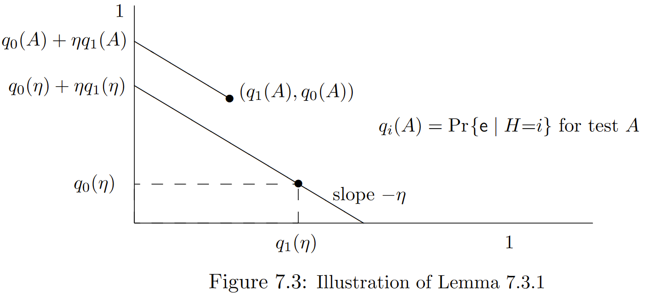
Proof: For any given \(\eta \), consider the a priori probabilities⁵ \((p_0, p_1)\) for which \(\eta = p_1/p_0\). The overall error probability for test \( A\) using these a priori probabilities is then

\[ \text{Pr\{e}(A)\} = p_0q_0 \ref{A} +p_1q_1(A) = p_0[q_0(A)+\eta q_1(A)] \nonumber \]

Similarly, the overall error probability for the threshold test \(\eta \) using the same a priori probabilities is

\[ \text{Pr\{e}(\eta) \} = p_0q_0(\eta ) +p_1q_1(\eta ) = p_0 [ q_0(\eta )+\eta q_1(\eta) ] \nonumber \]

This latter error probability is the MAP error probability for the given \(p_0, p_1\), and is thus the minimum overall error probability (for the given \( p_0, p_1\)) over all tests. Thus

\[ q_0(\eta ) + \eta q_1(\eta ) \leq q_0 \ref{A} + \eta q_1(A) \nonumber \]

As shown in the figure, these are the points at which the lines of slope \(−\eta \) from \((q_1(A), q_0(A))\) and \((q_1(\eta ), q_0(\eta ))\) respectively cross the ordinate axis. Thus all points on the first line (including \((q_1(A), q_0(A)))\) lie in the closed half plane above and to the right of all points on the second, completing the proof.

\(\square \)

The straight line of slope \( −\eta \) through the point \( (q_1(\eta ), q_0(\eta ))\) has the equation \( f_{\eta}(\alpha) = q_0(\eta) + \eta (q_1(\eta ) − \alpha)\). Since the lemma is valid for all \(\eta , 0 < \eta < \infty \), the point \((q_1(A), q_0(A))\) for an arbitrary test lies above and to the right of the entire family of straight lines that, for each \(\eta \), pass through \((q_1(\eta ), q_0(\eta ))\) with slope \(-\eta \). This family of straight lines has an upper envelope called the error curve, \(u(\alpha)\), defined by

\[ u(\alpha ) = \sup_{0\leq \eta < \infty} q_0(\eta )+\eta (q_1(\eta )-\alpha ) \nonumber \]

The lemma then asserts that for every test \(A\) (including threshold tests), we have \(u(q_1(A)) \leq q_0(A)\). Also, since every threshold test lies on one of these straight lines, and therefore on or below the curve \(u(\alpha )\), we see that the error probabilities \((q_1(\eta ), q_0(\eta)\) for each threshold test must lie on the curve \(u(\alpha )\). Finally, since each straight line defining \(u(\alpha )\) forms a tangent of \( u(\alpha )\) and lies on or below \(u(\alpha )\), the function \(u(\alpha )\) is convex.⁶ Figure 7.4 illustrates the error curve.

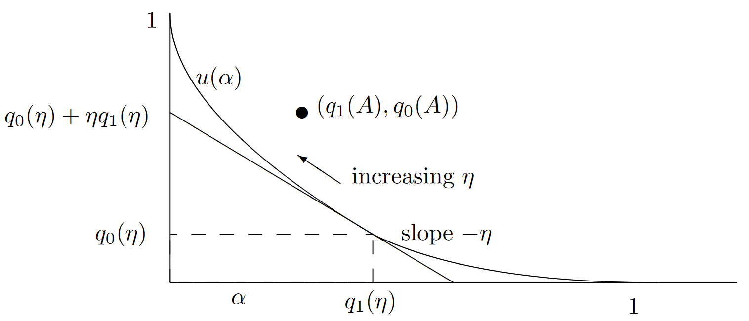
Figure 7.4: Illustration of the error curve \(u(\alpha )\) (see (7.3.7)). Note that \(u(\alpha )\) is convex, lies on or above its tangents, and on or below all tests. It can also be seen, either directly from the curve above or from the definition of a threshold test, that \(q_1(\eta )\) is non-increasing in \(\eta\) and \(q_0(\eta )\) is non-decreasing.

The error curve essentially gives us a tradeoff between the probability of error given \(H = 0\) and that given \(H = 1\). Threshold tests, since they lie on the error curve, provide optimal points for this tradeoff.

The argument above lacks one important feature. Although all threshold tests lie on the error curve, we have not shown that all points on the error curve correspond to threshold tests. In fact, as the following example shows, it is sometimes necessary to generalize threshold tests by randomization in order to reach all points on the error curve.

Before proceeding to this example, note that Lemma 7.3.1 and the definition of the error curve apply to a broader set of models than discussed so far. First, the lemma still holds if \(f_{\boldsymbol{Y} |H} (\boldsymbol{y} | \ell )\) is zero over an arbitrary set of \(\boldsymbol{y}\) for one or both hypotheses \(\ell \). The likelihood ratio \(\Lambda (\boldsymbol{y})\) is infinite where \( f_{\boldsymbol{Y} |H} (\boldsymbol{y} | 0) > 0\) and \(f_{\boldsymbol{Y} |H} (\boldsymbol{y} | 1) = 0\), but this does not affect the proof of the lemma. Exercise 7.6 helps explain how this situation can affect the error curve.

In addition, it can be seen that the lemma also holds if \(\boldsymbol{Y}\) is an \(n\)-tuple of discrete rv’s. The following example further explains the discrete case and also shows why not all points on the error curve correspond to threshold tests. What we assume throughout is that \(\Lambda(\boldsymbol{Y} )\) is a rv conditional on \(H = 1\) and is a possibly-defective⁷ rv conditional on \( H = 0\).

Example 7.3.2 About the simplest example of a detection problem is that with a one-dimensional binary observation Y . Assume then that

\[ \text{p}_{Y|H} \ref{0|0} = \text{p}_{Y|H}(1|1) = \dfrac{2}{3}; \qquad \text{p}_{Y|H}(0|1) = \text{p}_{Y|H}(1|0)=\dfrac{1}{3} \nonumber \]

Thus the observation \(Y\) equals \( H\) with probability 2/3. The ‘natural’ decision rule would be to select \(\hat{h}\) to agree with the observation \( y\), thus making an error with probability 1/3, both conditional on \(H = 1\) and \(H = 0\). It is easy to verify from (7.3.4) (using PMF’s in place of densities) that this ‘natural’ rule is the MAP rule if the a priori probabilities are in the range \(1/3 ≤ p_1 < 2/3\).

For \( p_1 < 1/3\), the MAP rule can be seen to be \(\hat{h} = 0\), no matter what the observation is. Intuitively, hypothesis 1 is too unlikely a priori to be overcome by the evidence when \(Y = 1\). Similarly, if \(p_1 ≥ 2/3\), then the MAP rule selects \(\hat{h} = 1\), independent of the observation.

The corresponding threshold test (see (7.3.6)) selects \(\hat{h} = y\) for \(1/2 ≤ \eta < 2\). It selects \(\hat{h} = 0\) for \(\eta < 1/2\) and \(\hat{h} = 1\) for \(\eta ≥ 2\). This means that, although there is a threshold test for each \(\eta\), there are only 3 resulting error probability pairs, \(i.e., \, (q_1(\eta ), q_0(\eta )\) can be (0, 1) or (1/3, 1/3), or (1, 0). The first pair holds for \(\eta ≥ 2\), the second for \(1/2 ≤ \eta < 2\), and the third for \(\eta< 1/2\). This is illustrated in Figure 7.5.

We have just seen that there is a threshold test for each \(\eta , \, 0 < \eta< \infty \), but those threshold tests map to only 3 distinct points \((q_1(\eta ), q_0(\eta ))\). As can be seen, the error curve joins these 3 points by straight lines.

Let us look more carefully at the tangent of slope -1/2 through the point (1/3, 1/3). This corresponds to the MAP test at \( \text{p}_1 = 1/3\). As seen in (7.3.4), this MAP test selects \(\hat{h} = 1\) for \(y = 1\) and \(\hat{h} = 0\) for \( y = 0\). The selection of \(\hat{h} = 1\) when \( y = 1\) is a don’t-care choice in which selecting \(\hat{h} = 0\) would yield the same overall error probability, but would change \((q_1(\eta ), q_0(\eta )\) from (1/3, 1/3) to (1, 0).

It is not hard to verify (since there are only 4 tests, \(i.e.\), deterministic rules, for mapping a binary variable to another binary variable) that no test can achieve the tradeoff between \(q_1(A)\) and \(q_0(A)\) indicated by the interior points on the straight line between (1/3, 1/3) and (1, 0). However, if we use a randomized rule, mapping 1 to 1 with probability \(\theta\) and into 0 with probability \(1 − \theta\) (along with always mapping 0 to 0), then all points on the straight line from (1/3, 1/3) to (1, 0) are achieved as \(\theta\) goes from 0 to 1. In other words, a don’t-care choice for MAP becomes an important choice in the tradeoff between \(q_1(A)\) and \(q_0(A)\).

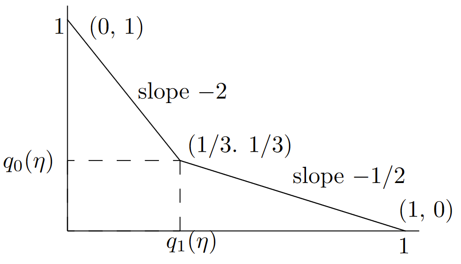
Figure 7.5: Illustration of the error curve \(u(\alpha )\) for Example 7.3.2. For all \(\eta \) in the range \(1/2 ≤ \eta < 2\), the threshold test selects \(\hat{h} = y\). The corresponding error probabilities are then \(q_1(\eta ) = q_0(\eta ) = 1/3\). For \(\eta< 1/2\), the threshold test selects \(\hat{h} = 0\) for all \( y\), and for \(\eta > 2\), it selects \(\hat{h} = 1\) for all \(y\). The error curve (see (7.3.7)) for points to the right of (1/3, 1/3) is maximized by the straight line of slope -1/2 through (1/3, 1/3). Similarly, the error curve for points to the left of (1/3, 1/3) is maximized by the straight line of slope -2 through (1/3, 1/3). One can visualize the tangent lines as an inverted see-saw, first see-sawing around (0,1), then around (1/3, 1/3), and finally around (1, 0).

In the same way, all points on the straight line from (0, 1) to (1/3, 1/3) can be achieved by a randomized rule that maps 0 to 0 with given probability \(\theta\) (along with always mapping 1 to 1).

In the general case, the error curve can contain straight line segments whenever the distribu­tion function of the likelihood ratio, conditional on \(H = 1\), is discontinuous. This is always the case for discrete observations, and, as illustrated in Exercise 7.6, might also occur with continuous observations. To understand this, suppose that Pr{\(\Lambda (\boldsymbol{Y} ) = \eta | H=1\} = \beta > 0\) for some \(\eta , 0 < \eta < 1\). Then the MAP test at \(\eta \) has a don’t-care region of probability \(\beta \) given \( H = 1\). This means that if the MAP test is changed to resolve the don’t-care case in favor of \(H = 0\), then the error probability \(q_1\) is increased by \(\beta\) and the error probability \(q_0\) is decreased by \(\eta \beta\). Lemma 7.3.1 is easily seen to be valid whichever way the don’t-care cases are resolved, and thus both \( (q_1, q_0)\) and \( (q_1+\beta, q_0−\eta \beta)\) lie on the error curve. Since all tests lie above and to the right of the straight line of slope \(−\eta \) through these points, the error curve has a straight line segment between these points. As mentioned before, any pair of error probabilities on this straight line segment can be realized by using a randomized threshold test at \(\eta \).

The Neyman-Pearson rule is the rule (randomized where needed) that realizes any desired error probability pair \((q_1, q_0)\) on the error curve, \(i.e\)., where \(q_0 = u(q_1)\). To be specific, as­sume the constraint that \(q_1 = \alpha\) for any given \(\alpha , \, 0 < \alpha ≤ 1\). Since Pr{\(\Lambda (\boldsymbol{Y}) > \eta | H = 1\)} is a complementary distribution function, it is non-increasing in \(\eta \), perhaps with step dis­continuities. At \(\eta = 0\), it has the value 1−Pr{\(\Lambda (\boldsymbol{Y} ) = 0\)}. As \(\eta \) increases, it decreases to 0, either for some finite \(\eta \) or as \(\eta \rightarrow \infty\). Thus if \(0 < \alpha ≤ 1 − \text{Pr}\{ \Lambda (\boldsymbol{Y} ) = 0\)}, we see that \(\alpha \) is either equal to Pr{\(\Lambda (\boldsymbol{y}) > \eta | H = 1\)} for some \(\eta \) or \(\alpha \) is on a step discontinuity at some \(\eta \). Defining \(\eta (\alpha )\) as an \(\eta \) where one of these alternatives occur,⁸ there is a solution to the following:

\[ \text{Pr} \{ \Lambda (\boldsymbol{y})>\eta (\alpha ) |H=1\} \leq \alpha \leq \text{Pr}\{ \Lambda (\boldsymbol{y}) \geq \eta (\alpha ) | H=1 \} \nonumber \]

Note that (7.3.8) also holds, with \(\eta (\alpha ) = 0\) if \(1 − \text{Pr}\{ \Lambda (\boldsymbol{Y} )=0 \} < \alpha ≤ 1. \)

The Neyman-Pearson rule, given \(\alpha \), is to use a threshold test at \(\eta (\alpha )\) if Pr{\(\Lambda (\boldsymbol{y} )=\eta (\alpha ) | H=1 \} = 0\). If Pr\(\{ \Lambda (\boldsymbol{y} )=\eta (\alpha ) | H=1\} > 0\), then a randomized test is used at \(\eta (\alpha )\). When \(\Lambda (\boldsymbol{y} ) = \eta (\alpha ), \, \hat{h}\) is chosen to be 1 with probability \(\theta \) where

\[ \theta = \dfrac{\alpha - \text{Pr} \{ \Lambda (\boldsymbol{y} )>\eta (\alpha )|H=1\} }{\text{Pr} \{ \Lambda (\boldsymbol{y} ) = \eta (\alpha ) | H=1\} } \nonumber \]

This is summarized in the following theorem:

Theorem 7.3.1. Assume that the likelihood ratio \(\Lambda (\boldsymbol{Y})\) is a rv under \( H = 1\). For any \(\alpha ,\, 0 < \alpha \leq 1\), the constraint that Pr{\(\text{e} | H = 1\} \leq \alpha \) implies that Pr{\(\text{e} | H = 0\} \geq u(\alpha )\) where \(u(\alpha )\) is the error curve. Furthermore, Pr{\(\text{e} | H = 0\} = u(\alpha )\) if the Neyman-Pearson rule, specified in (7.3.8) and (7.3.9), is used.

Proof: We have shown that the Neyman-Pearson rule has the stipulated error probabilities. An arbitrary decision rule, randomized or not, can be specified by a finite set \(A_1, . . . , A_k\) of deterministic decision rules along with a rv \( V\), independent of \(H\) and \(\boldsymbol{Y}\), with sample values \(1, . . . , k\). Letting the PMF of \(V\) be \( (θ_1, . . . , θ_k)\), an arbitrary decision rule, given \(\boldsymbol{Y} = \boldsymbol{y}\) and \(V = i\) is to use decision rule \(A_i\) if \(V = i\). The error probabilities for this rule are Pr{\(\text{e} | H=1\} = \sum^k_{i=1} θ_iq_1(A_i)\) and Pr{\(\text{e} | H=0\} = \sum^k_{i=1} θ_iq_0(A_i)\). It is easy to see that Lemma 7.3.1 applies to these randomized rules in the same way as to deterministic rules.

\( \square \)

All of the decision rules we have discussed are threshold rules, and in all such rules, the first part of the decision rule is to find the likelihood ratio \(\Lambda (\boldsymbol{y})\) from the observation \(\boldsymbol{y}\). This simplifies the hypothesis testing problem from processing an \(n\)-dimensional vector \(\boldsymbol{y}\) to processing a single number \(\Lambda (\boldsymbol{y})\), and this is typically the major component of making a threshold decision. Any intermediate calculation from \(\boldsymbol{y}\) that allows \(\Lambda (\boldsymbol{y} )\) to be calculated is called a sufficient statistic. These usually play an important role in detection, especially for detection in noisy environments.

There are some hypothesis testing problems in which threshold rules are in a sense inappro­priate. In particular, the cost of an error under one or the other hypothesis could be highly dependent on the observation \(boldsymbol{y}\). A minimum cost threshold test for each \(\boldsymbol{y}\) would still be appropriate, but a threshold test based on the likelihood ratio might be inappropriate since different observations with very different cost structures could have the same likelihood ratio. In other words, in such situations, the likelihood ratio is no longer sufficient to make a minimum cost decision.

So far we have assumed that a decision is made after a predetermined number \(n\) of obser­vations. In many situations, observations are costly and introduce an unwanted delay in decisions. One would prefer, after a given number of observations, to make a decision if the resulting probability of error is small enough, and to continue with more observations otherwise. Common sense dictates such a strategy, and the branch of probability theory analyzing such strategies is called sequential analysis. In a sense, this is a generalization of Neyman-Pearson tests, which employed a tradeoff between the two types of errors. Here we will have a three-way tradeoff between the two types of errors and the time required to make a decision.

We now return to the hypothesis testing problem of major interest where the observations, conditional on the hypothesis, are IID. In this case the log-likelihood ratio after n observa­tions is the sum \(S_n = Z_1 + Z_n\) of the \(n\) IID individual log likelihood ratios. Thus, aside ··· from the question of making a decision after some number of observations, the sequence of log-likelihood ratios \(S_1, S_2, . . .\) is a random walk.

Essentially, we will see that an appropriate way to choose how many observations to make, based on the result of the earlier observations, is as follows: The probability of error under either hypothesis is based on \( S_n = Z_1 + ...+ Z_n\). Thus we will see that an appropriate rule is to choose \(H=0\) if the sample value \(s_n\) of \( S_n\) is more than some positive threshold \(\alpha\), to choose H₁ if \( s_n ≤ \beta\) for some negative threshold \(\beta\), and to continue testing if the sample value has not exceeded either threshold. In other words, the decision time for these sequential decision problems is the time at which the corresponding random walk crosses a threshold. An error is made when the wrong threshold is crossed.

We have now seen that both the queueing delay in a G/G/1 queue and the above sequential hypothesis testing problem can be viewed as threshold crossing problems for random walks. The following section begins a systemic study of such problems.

_____________________________________

1. Statisticians have argued since the earliest days of statistics about the ‘validity’ of choosing a priori probabilities for the hypotheses to be tested. Bayesian statisticians are comfortable with this practice and non-Bayesians are not. Both are comfortable with choosing a probability model for the observations conditional on each hypothesis. We take a Bayesian approach here, partly to take advantage of the power of a complete probability model, and partly because non-Bayesian results, \(i.e.\), results that do not depend on the a priori probabilies, are often easier to derive and interpret within a collection of probability models using different choices for the a priori probabilities. As will be seen, the Bayesian approach also makes it natural to incorporate the results of earlier observations into updated a priori probabilities for analyzing later observations. In defense of non-Bayesians, note that the results of statistical tests are often used in areas of significant public policy disagreement, and it is important to give the appearance of a lack of bias. Statistical results can be biased in many more subtle ways than the use of a priori probabilities, but the use of an a priori distribution is particularly easy to attack.
2. In a sense, it is in making decisions where the rubber meets the road. For real-world situations, a probabilistic analysis is often connected with studying the problem, but eventually one technology or another must be chosen for a system, one person or another must be hired for a job, one law or another must be passed, etc.
3. Note that in a non-Bayesian formulation, \(\boldsymbol{Y}\) is a different random vector, in a different probability space, for \(H = 0\) than for \(H = 1\). However, the corresponding conditional probabilities for each exist in each probability space, and thus \(\Lambda (\boldsymbol{Y} )\) exists (as a different rv) in each space.
4. By assumption, the decision must be made on the basis of the observation \(\boldsymbol{y}\), so a deterministic rule is based solely on \(\boldsymbol{y},\, i.e.\), is a function of \(\boldsymbol{y}\). We will see later that randomized rather than deterministic rules are required for some purposes, but such rules are called randomized rules rather than tests.
5. Note that the lemma does not assume any a priori probabilities. The MAP test for each a priori choice \((p_0, p_1)\) determines \(q_0(\eta )\) and \(q_1(\eta )\) for \(\eta = p_1/p_0\). Its interpretation as a MAP test depends on a model with a priori probabilities, but its calculation depends only on \(p_0, p_1\) viewed as parameters.
6. A convex function of a real variable is sometimes defined as a function with a nonnegative second derivative, but defining it as a function lying on or above all its tangents is more general, allowing for step discontinuities in the first derivative of \( f\). We see the need for this generality shortly.
7. If \(\text{p}_{\boldsymbol{Y} |H} (\boldsymbol{y} | 1) = 0\) and \(\text{p}_{\boldsymbol{Y} |H (\boldsymbol{y} | 0) > 0\) for some \(\boldsymbol{y}\), then \(\Lambda (\boldsymbol{y})\) is infinite, and thus defective, conditional on \(H = 0\). Since the given \(\boldsymbol{y}\) has zero probability conditional on \(H = 0\), we see that \(\Lambda (\boldsymbol{Y} )\) is not defective conditional on \(H = 1\).
8. In the discrete case, there can be multiple solutions to (7.3.8) for some values of \(\alpha \), but this does not affect the decision rule. One can choose the smallest value of \(\eta \) to satisfy (7.3.8) if one wants to eliminate this ambiguity.