7.12: Exercises

Exercise 7.1. Consider the simple random walk {\(S_n; n ≥ 1\)} of Section 7.1.1 with \(S_n = X_1 + ··· + X_n\) and \(\text{Pr}\{X_i = 1\} = p; \text{ Pr}\{X_i = −1\} = 1 − p\); assume that \(p ≤ 1/2\).

a) Show that \(\text{Pr}\left\{ \bigcup_{n\geq 1} \{S_n ≥ k\} \right\}=\left[\text{Pr}\left\{ \bigcup_{n≥1} \{ S_n ≥1 \} \right\} \right]^k\) for any positive integer \(k\). Hint: Given that the random walk ever reaches the value 1, consider a new random walk starting at that time and explore the probability that the new walk ever reaches a value 1 greater than its starting point.

b) Find a quadratic equation for \(y = \text{Pr}\left\{\bigcup_{n≥1} \{S_n ≥ 1\}\right\}\). Hint: explore each of the two possibilities immediately after the first trial.

c) For \(p < 1/2\), show that the two roots of this quadratic equation are \(p/(1 − p)\) and 1. Argue that \(\text{Pr}\left\{\bigcup_{n≥1} \{S_n ≥ 1\}\right\}\) cannot be 1 and thus must be \(p/(1 − p)\).

d) For \(p = 1/2\), show that the quadratic equation in part c) has a double root at 1, and thus \(\text{Pr}\left\{ \bigcup_{n≥1} \{S_n ≥ 1\}\right\} = 1\). Note: this is the very peculiar case explained in the section on Wald’s equality.

e) For \( p < 1/2\), show that \(p/(1 − p) = \exp(−r^∗)\) where \(r^∗\) is the unique positive root of \(g(r) = 1\) where \(g(r) = \mathsf{E} [e^{rX}]\).

Exercise 7.2. Consider a G/G/1 queue with IID arrivals {\(X_i; i ≥ 1\)}, IID FCFS service times {\(Y_i; i ≥ 0\)}, and an initial arrival to an empty system at time 0. Define \(U_i = X_i −Y_{i−1}\) for \(i ≥ 1\). Consider a sample path where \((u_1, . . . , u_6) = (1, −2, 2, −1, 3, −2)\).

a) Let \(Z_i^6 = U_6 + U_{6−1} + . . . + U_{6−i+1}\). Find the queueing delay for customer 6 as the max­imum of the ‘backward’ random walk with elements \(0, Z_1^6, Z_2^6, . . . , Z_6^6\); sketch this random walk.

b) Find the queueing delay for customers 1 to 5.

c) Which customers start a busy period (\(i.e.\), arrive when the queue and server are both
empty)? Verify that if \(Z_i^6\) maximizes the random walk in part a), then a busy period starts
with arrival \(6 − i\).

d) Now consider a forward random walk \(V_n = U_1 +... +U_n\). Sketch this walk for the sample path above and show that the queueing delay for each customer is the difference between two appropriately chosen values of this walk.

Exercise 7.3. A G/G/1 queue has a deterministic service time of 2 and interarrival times that are 3 with probability \(p\) and 1 with probability \(1 − p\).

a) Find the distribution of \(W_1\), the wait in queue of the first arrival after the beginning of a busy period.

b) Find the distribution of \(W_{\infty}\), the steady-state wait in queue.

c) Repeat parts a) and b) assuming the service times and interarrival times are exponentially distributed with rates \( μ\) and \(\lambda \) respectively.

Exercise 7.4. A sales executive hears that one of his sales people is routing half of his incoming sales to a competitor. In particular, arriving sales are known to be Poisson at rate one per hour. According to the report (which we view as hypothesis 1), each second arrival is routed to the competition; thus under hypothesis 1 the interarrival density for successful sales is \(f (y|\mathsf{H}_1) = ye^{−y}; y ≥ 0\). The alternate hypothesis (\(\mathsf{H}_0\)) is that the rumor is false and the interarrival density for successful sales is \(f (y|\mathsf{H}_0) = e^{−y}; y ≥ 0\). Assume that, a priori, the hypotheses are equally likely. The executive, a recent student of stochastic processes, explores various alternatives for choosing between the hypotheses; he can only observe the times of successful sales however.

a) Starting with a successful sale at time 0, let \(S_i\) be the arrival time of the \(i^{th}\) subse­quent successful sale. The executive observes \(S_1, S_2, . . . , S_n(n ≥ 1)\) and chooses the maxi­mum aposteriori probability hypothesis given this data. Find the joint probability density \(f (S_1, S_2, . . . , S_n|\mathsf{H}_1)\) and \(f (S_1, . . . , S_n|\mathsf{H}_0)\) and give the decision rule.

b) This is the same as part a) except that the system is in steady state at time 0 (rather than starting with a successful sale). Find the density of \( S_1\) (the time of the first arrival after time 0) conditional on \(\mathsf{H}_0\) and on \(\mathsf{H}_1\). What is the decision rule now after observing \(S_1, . . . , S_n\).

c) This is the same as part b), except rather than observing n successful sales, the successful sales up to some given time \(t\) are observed. Find the probability, under each hypothesis, that the first successful sale occurs in \((s_1, s_1 + ∆]\), the second in \((s_2, s_2 + ∆], . . . ,\) and the last in \((s_{N (t)}, s_{N (t)} + ∆]\) (assume \(∆\) very small). What is the decision rule now?

Exercise 7.5. For the hypothesis testing problem of Section 7.3, assume that there is a cost \(C_0\) of choosing \(\mathsf{H}_1\) when \(\mathsf{H}_0\) is correct, and a cost \(C_1\) of choosing \(\mathsf{H}_0\) when \(\mathsf{H}_1\) is correct. Show that a threshold test minimizes the expected cost using the threshold \(η = (C_1p_1)/(C_0p_0)\).

Exercise 7.6. Consider a binary hypothesis testing problem where \(H\) is 0 or 1 and a one dimensional observation \(Y\) is given by \(Y = H + U\) where \(U\) is uniformly distributed over \([-1, 1]\) and is independent of \(H\).

a) Find \(\mathsf{f}_{Y |H} (y | 0), \mathsf{f}_{Y |H} (y | 1)\) and the likelihood ratio \(Λ(y)\).

b) Find the threshold test at \(η\) for each \(η, 0 < η<\infty\) and evaluate the conditional error probabilities, \(q_0(η)\) and \(q_1(η)\).

c) Find the error curve \( u(α)\) and explain carefully how \(u(0)\) and \(u(1/2)\) are found (hint: \(u(0) = 1/2\)).

d) Describe a decision rule for which the error probability under each hypothesis is 1/4. You need not use a randomized rule, but you need to handle the don’t-care cases under the threshold test carefully.

Exercise 7.7. a) For given \(α\), \(0 < α ≤ 1\), let \(η^∗\) achieve the supremum \(\sup_{0\leq \eta <\infty} q_1 (η) + η(q_0(η) − α)\). Show that \(η^∗ ≤ 1/α\). Hint: Think in terms of Lemma 7.3.1 applied to a very simple test.

b) Show that the magnitude of the slope of the error curve \(u(α)\) at \(α\) is at most \(1/α\).

Exercise 7.8. Define \(\gamma (r)\) as \(\ln [\mathsf{g}(r)]\) where \(\mathsf{g}(r) = \mathsf{E} [\exp (rX)]\). Assume that \(X\) is discrete with possible outcomes {\(a_i; i ≥ 1\)}, let \(p_i\) denote \(\text{Pr}\{X = a_i\}\), and assume that \(\mathsf{g}(r)\) exists in some open interval (\(r_- , r_+\)) containing \(r = 0\). For any given \(r\), \( r_- < r < r_+\), define a random variable \(X_r\) with the same set of possible outcomes {\(a_i; i ≥ 1\)} as \(X\), but with a probability mass function \(q_i = \text{Pr}\{X_r = a_i\} = p_i \exp[a_i r − \gamma (r)]\). \( X_r\) is not a function of \(X\), and is not even to be viewed as in the same probability space as \(X\); it is of interest simply because of the behavior of its defined probability mass function. It is called a tilted random variable relative to \(X\), and this exercise, along with Exercise 7.9 will justify our interest in it.

a) Verify that \(\sum_i q_i = 1\).

b) Verify that \(\mathsf{E} [X_r] = \sum_i a_iq_i\) is equal to \(\gamma'(r)\).

c) Verify that Var \([X_r] = \sum_i a_i^2 q_i − (\mathsf{E} [X_r])^2\) is equal to \(\gamma''(r)\).

d) Argue that \(\gamma''(r) ≥ 0\) for all \(r\) such that \(\mathsf{g}(r)\) exists, and that \(\gamma''(r) > 0\) if \(\gamma''(0) > 0\).

e) Give a similar definition of \(X_r\) for a random variable \(X\) with a density, and modify parts a) to d) accordingly.

Exercise 7.9. Assume that \(X\) is discrete, with possible values {\(a_i; i ≥ 1\)) and probabilities \(\text{Pr}\{X = a_i\} = p_i\). Let \(X_r\) be the corresponding tilted random variable as defined in Exercise 7.8. Let \(S_n = X_1 +... + X_n\) be the sum of \( n\) IID rv’s with the distribution of \(X\), and let \(S_{n,r} = X_{1,r} + ...+ X_{n,r}\) be the sum of \(n\) IID tilted rv’s with the distribution of \(X_r\). Assume that \(\overline{X} < 0\) and that \( r > 0\) is such that \(\gamma (r)\) exists.

a) Show that \(\text{Pr}\{S_{n,r} =s\} = \text{Pr}\{S_n =s\} \exp[sr − n\gamma (r)]\). Hint: first show that

\[ \text{Pr}\{ X_{1,r}=v_1,...,X_{n,r}=v_n \} = \text{Pr}\{X_1=v_1,...,X_n=v_n\} \exp [sr-n\gamma (r)] \nonumber \]

where \(s=v_1+...+v_n\).

b) Find the mean and variance of \(S_{n,r}\) in terms of \(\gamma(r)\).

c) Define \(a= \gamma'(r)\) and \(σ_r^2 = \gamma''(r)\). Show that \(\text{Pr}\left\{| S_{n,r} − na|≤\sqrt{2n}σ_r\right\} > 1/2\). Use this to show that

\[\text{Pr} \left\{ \left| S_n-na \right| \leq \sqrt{2n}\sigma_r \right\} > (1/2)\exp [-r(an+\sqrt{2n} \sigma_r ) +n\gamma (r)] \nonumber \]

d) Use this to show that for any \(\epsilon\) and for all sufficiently large \(n\),

\[ \text{Pr}\{ S_n\geq n(\gamma'(r)-\epsilon)\}>\dfrac{1}{2}\exp [-rn(\gamma' (r)+\epsilon )+n\gamma (r)] \nonumber \]

Exercise 7.10. Consider a random walk with thresholds \( α> 0\), \(β< 0\). We wish to find \(\text{Pr}\{S_J ≥ α\}\) in the absence of a lower threshold. Use the upper bound in (7.5.9) for the probability that the random walk crosses \(α\) before \(β\).

a) Given that the random walk crosses \(β\) first, find an upper bound to the probability that \(α\) is now crossed before a yet lower threshold at \(2β\) is crossed.

b) Given that \( 2β\) is crossed before \(α\), upperbound the probability that \(α\) is crossed before a threshold at \(3β\). Extending this argument to successively lower thresholds, find an upper bound to each successive term, and find an upper bound on the overall probability that \(α\) is crossed. By observing that \(β\) is arbitrary, show that (7.5.9) is valid with no lower threshold.

Exercise 7.11. This exercise verifies that Corollary 7.5.1 holds in the situation where \(\gamma(r) < 0\) for all \(r ∈ (r_−, r_+)\) and where \(r^∗\) is taken to be \(r_+\) (see Figure 7.7).

a) Show that for the situation above, \(\exp (rS_J ) ≤ \exp(rS_J − J\gamma (r))\) for all \(r ∈ (0, r^∗)\).

b) Show that \(\mathsf{E} [\exp (rS_J )] ≤ 1\) for all \(r ∈ (0, r^∗)\).

c) Show that \(\text{Pr}\{S_J ≥ α\}≤ \exp(−rα)\) for all \(r ∈ (0, r^∗)\). Hint: Follow the steps of the proof of Corollary 7.5.1.

d) Show that \(\text{Pr}\{ S_J ≥ α\} ≤ \exp(−r^∗α)\).

Exercise 7.12. a) Use Wald’s equality to show that if \(\overline{X} = 0\), then \(\mathsf{E} [S_J ] = 0\) where \(J\) is the time of threshold crossing with one threshold at \(α> 0\) and another at \(β< 0\).

b) Obtain an expression for \(\text{Pr}\{S_J ≥ α\}\). Your expression should involve the expected value of \(S_J\) conditional on crossing the individual thresholds (you need not try to calculate these expected values).

c) Evaluate your expression for the case of a simple random walk.

d) Evaluate your expression when \(X\) has an exponential density, \(\mathsf{f}_X \ref{x} = a_1e^{−\lambda x}\) for \(x ≥ 0\) and \(\mathsf{f}_X \ref{x} = a_2e^{μx}\) for \(x < 0\) and where \(a_1\) and \(a_2\) are chosen so that \(\overline{X} = 0\).

Exercise 7.13. A random walk {\(S_n; n ≥ 1\)}, with \(S_n =\sum^n_{i=1} X_i\), has the following probability density for \(X_i\)

\[ \mathsf{f}_X(x) = \left\{ \begin{array}{pp} \dfrac{e^{-x}}{e-e^{-1}} \,; \qquad -1\leq x \leq 1 \\ \\ \\ =0 \,; \qquad \text{elsewhere} \end{array} \right. \nonumber \]

a) Find the values of \( r\) for which \(\mathsf{g}(r) = \mathsf{E} [\exp (rX)] = 1\).

b) Let \( P_α\) be the probability that the random walk ever crosses a threshold at \(α\) for some \(α> 0\). Find an upper bound to \(P_α\) of the form \(P_α ≤ e^{−αA}\) where \(A\) is a constant that does not depend on \(α\); evaluate \(A\).

c) Find a lower bound to \(P_α\) of the form \(P_α ≥ Be^{−αA}\) where \(A\) is the same as in part b) and \(B\) is a constant that does not depend on \(α\). Hint: keep it simple — you are not expected to find an elaborate bound. Also recall that \(\mathsf{E}[e^{r^∗S_J} ]= 1\) where \(J\) is a stopping trial for the random walk and \(\mathsf{g}(r^∗) = 1\).

Exercise 7.14. Let {\(X_n; n ≥ 1\)} be a sequence of IID integer valued random variables with the probability mass function \(P_X \ref{k} = Q_k\). Assume that \(Q_k > 0\) for \(|k| ≤ 10\) and \(Q_k = 0\) for \(|k| > 10\). Let {\(S_n; n ≥ 1\)} be a random walk with \(S_n = X_1 + ··· + X_n\). Let \(α> 0\) and \(β< 0\) be integer valued thresholds, let \(J\) be the smallest value of \(n\) for which either \(S_n ≥ α\) or \(S_n ≤ β\). Let {\(S_n^∗; n ≥ 1\)} be the stopped random walk; \(i.e.\), \(S^∗_n= S_n\) for \(n ≤ J\) and \(S_n^∗= S_J\) for \(n > J\). Let \(π_i^∗ = \text{Pr}\{S_J = i\}\).

a) Consider a Markov chain in which this stopped random walk is run repeatedly until the point of stopping. That is, the Markov chain transition probabilities are given by \(P_{ij} = Q_{j−i}\) for \(β< i < α\) and \(P_{i0} = 1\) for \(i ≤ β\) and \(i ≥ α\). All other transition probabilities are 0 and the set of states is the set of integers \( [−9 + β, 9 + α]\). Show that this Markov chain is ergodic.

b) Let {\(π_i\)} be the set of steady-state probabilities for this Markov chain. Find the set of probabilities {\(π_i^∗\)} for the stopping states of the stopped random walk in terms of {\(π_i\)}.

c) Find \(\mathsf{E} [S_J ]\) and \(\mathsf{E} [J]\) in terms of {\(π_i\)}.

Exercise 7.15. a) Conditional on \(H_0\) for the hypothesis testing problem, consider the random variables \(Z_i = \ln [f (Y_i|\mathsf{H}_1)/f (Y_i|H_0)]\). Show that \(r^∗\), the positive solution to \(\mathsf{g}(r) = 1\), where \(g(r) = \mathsf{E} [\exp (rZi)]\), is given by \(r^∗ = 1\).

b) Assuming that \(Y\) is a discrete random variable (under each hypothesis), show that the tilted random variable \(Z_r\) with \(r = 1\) has the PMF \(P_Y (y|\mathsf{H}_1)\).

Exercise 7.16. a) Suppose {\(Z_n; n ≥ 1\)} is a martingale. Verify (7.6.13); \(i.e.\), \(\mathsf{E} [Z_n] = \mathsf{E} [Z_1]\) for \(n > 1\).

b) If {\(Z_n; n ≥ 1\)} is a submartingale, verify (7.7.5), and if a supermartingale, verify (7.7.6).

Exercise 7.17. Suppose {\(Z_n; n ≥ 1\)} is a martingale. Show that

\[ \mathsf{E}[Z_m|Z_{n_i},Z_{n_{i-1}},...,Z_{n_1}] = Z_{n_i} \text{ for all } 0<n_1<n_2<...<n_i <m \nonumber \]

Exercise 7.18. a) Assume that {\(Z_n; n ≥ 1\)} is a submartingale. Show that

\[\mathsf{E} [Z_m|Z_n,Z_{n-1},...,Z_1] \geq Z_n \text{ for all } n<m \nonumber \]

b) Show that

\[ \mathsf{E}[Z_m|Z_{n_i},Z_{n_{i-1}},...,Z_{n_1}] \geq Z_{n_i} \text{ for all } 0<n_1<n_2<...<n_i<m \nonumber \]

c) Assume now that {\(Z_n; n ≥ 1\)} is a supermartingale. Show that parts a) and b) still hold
with \( ≥\) replaced by \(≤\).

Exercise 7.19. Let {\(Z_n = \exp [rS_n − n\gamma (r)]; n ≥ 1\)} be the generating function martingale of (7.6.7) where \(S_n = X_1 +... + X_n\) and \(X_1, . . . X_n\) are IID with mean \(\overline{X} < 0\). Let \(J\) be the possibly-defective stopping trial for which the process stops after crossing a threshold at \(α> 0\) (there is no negative threshold). Show that \(\exp [r^∗α]\) is an upper bound to the probability of threshold crossing by considering the stopped process {\(Z_n^∗; n ≥ 1\)}.

The purpose of this exercise is to illustrate that the stopped process can yield useful upper bounds even when the stopping trial is defective.

Exercise 7.20. This problem uses martingales to find the expected number of trials \(\mathsf{E} [J]\) before a fixed pattern, \(a_1, a_2, . . . , a_k\), of binary digits occurs within a sequence of IID bi­nary random variables \(X_1, X_2, . . .\) (see Exercises 4.32 and 3.28 for alternate approaches). A mythical casino and set of gamblers who follow a prescribed strategy will be used to determine \(\mathsf{E} [J]\). The casino has a game where, on the \(i\)th trial, gamblers bet money on either 1 or 0. After bets are placed, \(X_i\) above is used to select the outcome 0 or 1. Let \(p(1) = \mathsf{p}_X (1)\) and \(p(0) = 1 − p(1) = \mathsf{p}_X (0)\). If an amount \(s\) is bet on 1, the casino receives \(s\) if \( X_i = 0\), and pays out \(s/p(1) − s\) (plus returning the bet \(s\)) if \(X_i = 1\). If \(s\) is bet on 0, the casino receives \(s\) if \(X_i = 1\), and pays out \(s/p(0) − s\) (plus the bet \(s\)) if \(X_i = 0\).

a) Assume an arbitrary pattern of bets by various gamblers on various trials (some gamblers might bet arbitrary amounts on 0 and some on 1 at any given trial). Let \(Y_i\) be the net gain of the casino on trial \(i\). Show that \(\mathsf{E} [Y_i] = 0\) (\(i.e.\), show that the game is fair). Let \(Z_n = Y_1 + Y_2 +... + Y_n\) be the aggregate gain of the casino over \(n\) trials. Show that for the given pattern of bets, {\(Z_n; n ≥ 1\)} is a martingale.

b) In order to determine \(\mathsf{E} [J]\) for a given pattern \(a_1, a_2, . . . , a_k\), we program our gamblers to bet as follows:

i) Gambler 1 has an initial capital of 1 which is bet on \(a_1\) at trial 1. If he wins, his capital grows to \(1/p(a_1)\), which is bet on \(a_2\) at trial 2. If he wins again, he bets his entire capital, \(1/[p(a_1)p(a_2)]\), on \(a_3\) at trial 3. He continues, at each trial \(i\), to bet his entire capital on \(a_i\) until he loses at some trial (in which case he leaves with no money) or he wins on \(k\) successive trials (in which case he leaves with \(1/[p(a_1) . . . p(a_k)]\).

ii) Gambler \(j, j > 1\), follows exactly the same strategy but starts at trial \(j\). Note that if the pattern \(a_1, . . . , a_k\) appears for the first time at \(J = n\), then gambler \(n − k + 1\) leaves at time \(n\) with capital \(1/[p(a_1) . . . p(a_k)]\) and gamblers \(j < n − k + 1\) all lose their capital.

Suppose the string \((a_1, . . . , a_k)\) is \((0, 1)\). Let for the above gambling strategy. Given that \(J = 3\) (\(i.e.\), that \(X_2 = 0\) and \(X_3 = 1\)), note that gambler 1 loses his money at either trial 1 or 2, gambler 2 leaves at time 3 with \(1/[p(0)p(1)]\) and gambler 3 loses his money at time 3. Show that \(Z_J = 3 − 1/[p(0)p(1)]\) given \(J = 3\). Find \(Z_J\) given \(J = n\) for arbitrary \(n ≥ 2\) (note that the condition \(J = n\) uniquely specifies \(Z_J \)).

c) Find \(\mathsf{E}[Z_J ]\) from part a). Use this plus part b) to find \(\mathsf{E} [J]\).

d) Repeat parts b) and c) using the string \((a_1, . . . , a_k) = (1, 1)\). Be careful about gambler 3 for \(J = 3\). Show that \(\mathsf{E} [J] = 1/[p(1)p(1)] + 1/p(1)\)

e) Repeat parts b) and c) for \((a_1, . . . , a_k) = (1, 1, 1, 0, 1, 1)\).

Exercise 7.21. a) This exercise shows why the condition \(\mathsf{E} [|Z_J |] < \infty\) is required in Lemma 7.8.1. Let \(Z_1 = −2\) and, for \(n ≥ 1\), let \(Z_{n+1} = Z_n[1 + X_n(3n + 1)/(n + 1)]\) where \(X_1, X_2, . . .\) are IID and take on the values \(+1\) and \(−1\) with probability 1/2 each. Show that {\(Z_n; n ≥ 1\)} is a martingale.

b) Consider the stopping trial \(J\) such that \(J\) is the smallest value of \(n > 1\) for which \(Z_n\) and \(Z_{n−1}\) have the same sign. Show that, conditional on \(n < J\), \(Z_n = (−2)^n/n\) and, conditional on \(n = J\), \(Z_J = −(−2)^n(n − 2)/(n^2 − n)\).

c) Show that \(\mathsf{E} [|Z_J |]\) is infinite, so that \(\mathsf{E} [Z_J ]\) does not exist according to the definition of expectation, and show that \(\lim_{n→\infty} \mathsf{E} [Z_n|J > n] \text{Pr}\{J > n\} = 0\).

Exercise 7.22. This exercise shows why the sup of a martingale can behave markedly differently from the maximum of an arbitrarily large number of the variables. More precisely, it shows that \(\text{Pr}\left\{ \sup_{n≥1} Z_n ≥ a\right\}\) can be unequal to \(\text{Pr}\left\{ \bigcup_{n≥1}\{Z_n ≥ a\}\right\}\).

a) Consider a martingale where \(Z_n\) can take on only the values \(2^{−n−1}\) and \(1 − 2^{−n−1}\), each with probability 1/2. Given that \(Z_n\), conditional on \(Z_{n−1}\), is independent of \(Z_1, . . . Z_{n−2}\), find \(\text{Pr}\{ Z_n|Z_{n−1}\}\) for each \(n\) so that the martingale condition is satisfied.

b) Show that \(\text{Pr}\left\{\sup_{n≥1} Z_n ≥ 1\right\} = 1/2\) and show that \(\text{Pr}\left\{ \bigcup_n \{Z_n ≥ 1\} \right\} = 0\).

c) Show that for every \(\epsilon > 0\), \(\text{Pr}\left\{ \sup_{n≥1} Z_n ≥ a\right\} ≤ \frac{\overline{Z}_1}{a-\epsilon }\). Hint: Use the relationship between \(\text{Pr}\left\{ \sup_{n≥1} Z_n ≥ a\right\}\) and \(\text{Pr}\left\{\bigcup_n\{Z_n ≥ a\}\right\}\) while getting around the issue in part b).

d) Use part c) to establish (7.9.3).

Exercise 7.23. Show that Theorem 7.7.1 is also valid for martingales relative to a joint process. That is, show that if \(h\) is a convex function of a real variable and if {\(Z_n; n ≥ 1\)} is a martingale relative to a joint process {\(Z_n, X_n; n ≥ 1\)}, then {\(h(Z_n); n ≥ 1\)} is a submartingale relative to {\(h(Z_n), X_n; n ≥ 1\)}.

Exercise 7.24. Show that if {\(Z_n; n ≥ 1\)} is a martingale (submartingale or supermartin­gale) relative to a joint process {\(Z_n, X_n; n ≥ 1\)} and if \(J\) is a stopping trial for {\(Z_n; n ≥ 1\)} relative to {\(Z_n, X_n; n ≥ 1\)}, then the stopped process is a martingale (submartingale or supermartingale) respectively relative to the joint process.

Exercise 7.25. Show that if {\(Z_n; n ≥ 1\)} is a martingale (submartingale or supermartin­gale) relative to a joint process {\(Z_n, X_n; n ≥ 1\)} and if \(J\) is a stopping trial for {\(Z_n; n ≥ 1\)} relative to {\(Z_n, X_n; n ≥ 1\)}, then the stopped process satisfies (7.8.3), (7.8.4), or (7.8.5) respectively.

Exercise 7.26. Show that if {\(Z_n; n\geq 1\)} is a martingale relative to a joint process {\(Z_n, X_n; n ≥1\)} and if \(J\) is a stopping trial for {\(Z_n; n ≥ 1\)} relative to {\(Z_n, X_n; n ≥ 1\)}, then \(\mathsf{E} [Z_J ] = \mathsf{E} [Z_1]\) if and only f (7.8.9) is satisfied.

Exercise 7.27. Consider the Markov modulated random walk in the figure below. The random variables \(Y_n\) in this example take on only a single value for each transition, that value being 1 for all transitions from state 1, 10 for all transitions from state 2, and 0 otherwise. \(\epsilon > 0\) is a very small number, say \(\epsilon < 10^{−6}\).

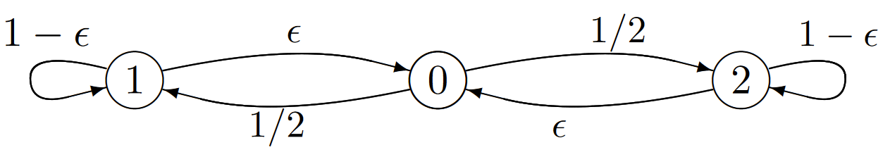
a) Show that the steady-state gain per transition is \(5.5/(1+ \epsilon)\). Show that the relative-gain vector is \(\boldsymbol{w} = (0, (\epsilon − 4.5)/[\epsilon (1 + \epsilon )]\), \((10\epsilon + 4.5)/[\epsilon (1 + \epsilon)])\).

b) Let \(S_n = Y_0 +Y_1 +... +Y_{n−1}\) and take the starting state \(X_0\) to be 0. Let \(J\) be the smallest value of \(n\) for which \(S_n ≥ 100\). Find \(\text{Pr}\{J = 11\}\) and \(\text{Pr}\{ J = 101\}\). Find an estimate of \(\mathsf{E} [J]\) that is exact in the limit \(\epsilon \rightarrow 0\).

c) Show that \(\text{Pr}\{ X_J = 1\} = (1 − 45\epsilon + o(\epsilon ))/2\) and that \(\text{Pr}\{ X_J = 2\} = (1 + 45\epsilon + o(\epsilon ))/2\). Verify, to first order in \(\epsilon \) that (7.10.17) is satisfied.

Exercise 7.28. Show that (7.10.17) results from taking the derivative of (7.10.21) and evalu­ating it at \(r = 0\).

Exercise 7.29. Let \(\{ Z_n; n ≥ 1\}\) be a martingale, and for some integer \(m\), let \(Y_n = Z_{n+m} −Z_m\).

a) Show that \(\mathsf{E} [Y_n | Z_{n+m−1} = z_{n+m−1}, Z_{n+m−2} = z_{n+m−2}, . . . , Z_m = z_m, . . . , Z_1 = z_1] = z_{n+m−1} − z_m\).

b) Show that \(\mathsf{E} [Y_n | Y_{n−1} = y_{n−1}, . . . , Y_1 = y_1] = y_{n−1}\).

c) Show that \(\mathsf{E} [|Y_n|] < \infty\). Note that b) and c) show that {\(Y_n; n ≥ 1\)} is a martingale.

Exercise 7.30. a) Show that Theorem 7.7.1 is valid if {\(Z_n; n ≥ 1\)} is a submartingale rather than a martingale. Hint: Simply follow the proof of Theorem 7.7.1 in the text.

b) Show that the Kolmogorov martingale inequality also holds if {\(Z_n; n ≥ 1\)} is a sub-martingale rather than a martingale.

Exercise 7.31 (Continuation of continuous-time branching) This exercise views the continuous-time branching process of Exercise 6.15 as a stopped random walk. Recall that the process was specified there as a Markov process such that for each state \(j\), \( j ≥ 0\), the transition rate to \(j + 1\) is \(j\lambda \) and to \(j − 1\) is \(jμ\). There are no other transitions, and in particular, there are no transitions out of state 0, so that the Markov process is reducible. Recall that the embedded Markov chain is the same as the embedded chain of an M/M/1 queue except that there is no transition from state 0 to state 1.

a) To model the possible extinction of the population, convert the embedded Markov chain above to a stopped random walk, {\(S_n; n ≥ 0\)}. The stopped random walk starts at \(S_0 = 0\) and stops on reaching a threshold at −1. Before stopping, it moves up by one with probability \(\frac{\lambda}{\lambda+μ}\) and downward by 1 with probability \(\frac{μ}{ \lambda+μ}\) at each step. Give the (very simple) relationship between the state \(X_n\) of the Markov chain and the state \(S_n\) of the stopped random walk for each \(n ≥ 0\).

b) Find the probability that the population eventually dies out as a function of \(\lambda\) and \(μ\). Be sure to consider all three cases \(\lambda > μ\), \(\lambda< μ\), and \(\lambda = μ\).