10.5: Adaptive Composition of FFT Algorithms

Last updated
Save as PDF

Page ID: 2025

$ \newcommand{\vecs}[1]{\overset { \scriptstyle \rightharpoonup} {\mathbf{#1}} } $

$ \newcommand{\vecd}[1]{\overset{-\!-\!\rightharpoonup}{\vphantom{a}\smash {#1}}} $

$ \newcommand{\id}{\mathrm{id}}$ $ \newcommand{\Span}{\mathrm{span}}$

( \newcommand{\kernel}{\mathrm{null}\,}\) $ \newcommand{\range}{\mathrm{range}\,}$

$ \newcommand{\RealPart}{\mathrm{Re}}$ $ \newcommand{\ImaginaryPart}{\mathrm{Im}}$

$ \newcommand{\Argument}{\mathrm{Arg}}$ $ \newcommand{\norm}[1]{\| #1 \|}$

$ \newcommand{\inner}[2]{\langle #1, #2 \rangle}$

$ \newcommand{\Span}{\mathrm{span}}$

$ \newcommand{\id}{\mathrm{id}}$

$ \newcommand{\Span}{\mathrm{span}}$

$ \newcommand{\kernel}{\mathrm{null}\,}$

$ \newcommand{\range}{\mathrm{range}\,}$

$ \newcommand{\RealPart}{\mathrm{Re}}$

$ \newcommand{\ImaginaryPart}{\mathrm{Im}}$

$ \newcommand{\Argument}{\mathrm{Arg}}$

$ \newcommand{\norm}[1]{\| #1 \|}$

$ \newcommand{\inner}[2]{\langle #1, #2 \rangle}$

$ \newcommand{\Span}{\mathrm{span}}$ $ \newcommand{\AA}{\unicode[.8,0]{x212B}}$

$ \newcommand{\vectorA}[1]{\vec{#1}} % arrow$

$ \newcommand{\vectorAt}[1]{\vec{\text{#1}}} % arrow$

$ \newcommand{\vectorB}[1]{\overset { \scriptstyle \rightharpoonup} {\mathbf{#1}} } $

$ \newcommand{\vectorC}[1]{\textbf{#1}} $

$ \newcommand{\vectorD}[1]{\overrightarrow{#1}} $

$ \newcommand{\vectorDt}[1]{\overrightarrow{\text{#1}}} $

$ \newcommand{\vectE}[1]{\overset{-\!-\!\rightharpoonup}{\vphantom{a}\smash{\mathbf {#1}}}} $

$ \newcommand{\vecs}[1]{\overset { \scriptstyle \rightharpoonup} {\mathbf{#1}} } $

$ \newcommand{\vecd}[1]{\overset{-\!-\!\rightharpoonup}{\vphantom{a}\smash {#1}}} $

$\newcommand{\avec}{\mathbf a}$ $\newcommand{\bvec}{\mathbf b}$ $\newcommand{\cvec}{\mathbf c}$ $\newcommand{\dvec}{\mathbf d}$ $\newcommand{\dtil}{\widetilde{\mathbf d}}$ $\newcommand{\evec}{\mathbf e}$ $\newcommand{\fvec}{\mathbf f}$ $\newcommand{\nvec}{\mathbf n}$ $\newcommand{\pvec}{\mathbf p}$ $\newcommand{\qvec}{\mathbf q}$ $\newcommand{\svec}{\mathbf s}$ $\newcommand{\tvec}{\mathbf t}$ $\newcommand{\uvec}{\mathbf u}$ $\newcommand{\vvec}{\mathbf v}$ $\newcommand{\wvec}{\mathbf w}$ $\newcommand{\xvec}{\mathbf x}$ $\newcommand{\yvec}{\mathbf y}$ $\newcommand{\zvec}{\mathbf z}$ $\newcommand{\rvec}{\mathbf r}$ $\newcommand{\mvec}{\mathbf m}$ $\newcommand{\zerovec}{\mathbf 0}$ $\newcommand{\onevec}{\mathbf 1}$ $\newcommand{\real}{\mathbb R}$ $\newcommand{\twovec}[2]{\left[\begin{array}{r}#1 \\ #2 \end{array}\right]}$ $\newcommand{\ctwovec}[2]{\left[\begin{array}{c}#1 \\ #2 \end{array}\right]}$ $\newcommand{\threevec}[3]{\left[\begin{array}{r}#1 \\ #2 \\ #3 \end{array}\right]}$ $\newcommand{\cthreevec}[3]{\left[\begin{array}{c}#1 \\ #2 \\ #3 \end{array}\right]}$ $\newcommand{\fourvec}[4]{\left[\begin{array}{r}#1 \\ #2 \\ #3 \\ #4 \end{array}\right]}$ $\newcommand{\cfourvec}[4]{\left[\begin{array}{c}#1 \\ #2 \\ #3 \\ #4 \end{array}\right]}$ $\newcommand{\fivevec}[5]{\left[\begin{array}{r}#1 \\ #2 \\ #3 \\ #4 \\ #5 \\ \end{array}\right]}$ $\newcommand{\cfivevec}[5]{\left[\begin{array}{c}#1 \\ #2 \\ #3 \\ #4 \\ #5 \\ \end{array}\right]}$ $\newcommand{\mattwo}[4]{\left[\begin{array}{rr}#1 \amp #2 \\ #3 \amp #4 \\ \end{array}\right]}$ $\newcommand{\laspan}[1]{\text{Span}\{#1\}}$ $\newcommand{\bcal}{\cal B}$ $\newcommand{\ccal}{\cal C}$ $\newcommand{\scal}{\cal S}$ $\newcommand{\wcal}{\cal W}$ $\newcommand{\ecal}{\cal E}$ $\newcommand{\coords}[2]{\left\{#1\right\}_{#2}}$ $\newcommand{\gray}[1]{\color{gray}{#1}}$ $\newcommand{\lgray}[1]{\color{lightgray}{#1}}$ $\newcommand{\rank}{\operatorname{rank}}$ $\newcommand{\row}{\text{Row}}$ $\newcommand{\col}{\text{Col}}$ $\renewcommand{\row}{\text{Row}}$ $\newcommand{\nul}{\text{Nul}}$ $\newcommand{\var}{\text{Var}}$ $\newcommand{\corr}{\text{corr}}$ $\newcommand{\len}[1]{\left|#1\right|}$ $\newcommand{\bbar}{\overline{\bvec}}$ $\newcommand{\bhat}{\widehat{\bvec}}$ $\newcommand{\bperp}{\bvec^\perp}$ $\newcommand{\xhat}{\widehat{\xvec}}$ $\newcommand{\vhat}{\widehat{\vvec}}$ $\newcommand{\uhat}{\widehat{\uvec}}$ $\newcommand{\what}{\widehat{\wvec}}$ $\newcommand{\Sighat}{\widehat{\Sigma}}$ $\newcommand{\lt}{<}$ $\newcommand{\gt}{>}$ $\newcommand{\amp}{&}$ $\definecolor{fillinmathshade}{gray}{0.9}$

As alluded to several times already, FFTW implements a wide variety of FFT algorithms (mostly rearrangements of Cooley-Tukey) and selects the “best” algorithm for a given $n$ automatically. In this section, we describe how such self-optimization is implemented, and especially how FFTW's algorithms are structured as a composition of algorithmic fragments. These techniques in FFTW are described in greater detail elsewhere, so here we will focus only on the essential ideas and the motivations behind them.

An FFT algorithm in FFTW is a composition of algorithmic steps called a plan. The algorithmic steps each solve a certain class of problems (either solving the problem directly or recursively breaking it into sub-problems of the same type). The choice of plan for a given problem is determined by a planner that selects a composition of steps, either by runtime measurements to pick the fastest algorithm, or by heuristics, or by loading a pre-computed plan. These three pieces: problems, algorithmic steps, and the planner, are discussed in the following subsections.

The problem to be solved

In early versions of FFTW, the only choice made by the planner was the sequence of radices, and so each step of the plan took a DFT of a given size $n$, possibly with discontiguous input/output, and reduced it (via a radix $r " role="presentation" style="position:relative;" tabindex="0">$ $\mathbf{O}[\mathbf{ko}]\; \text{for}\; 0\leq k< n$. However, we soon found that we could not easily express many interesting algorithms within this framework; for example, in-place $(\mathbf{I}=\mathbf{O})$ FFTs that do not require a separate bit-reversal stage. It became clear that the key issue was not the choice of algorithms, as we had first supposed, but the definition of the problem to be solved. Because only problems that can be expressed can be solved, the representation of a problem determines an outer bound to the space of plans that the planner can explore, and therefore it ultimately constrains FFTW's performance.

$(n,\mathbf{I},\imath ,\mathbf{O},o)$ problem definition was that it forced each algorithmic step to address only a single DFT. In fact, FFTs break down DFTs into multiple smaller DFTs, and it is the combination of these smaller transforms that is best addressed by many algorithmic choices, especially to rearrange the order of memory accesses between the subtransforms. Therefore, we redefined our notion of a problem in FFTW to be not a single DFT, but rather a loop of DFTs, and in fact multiple nested loops of DFTs. The following sections describe some of the new algorithmic steps that such a problem definition enables, but first we will define the problem more precisely.

\[\text{dft}(\mathbf{N},\mathbf{V},\mathbf{I}+k.\imath ,\mathbf{O}+k.o) \nonumber \]

The case of multi-dimensional DFTs is defined more precisely elsewhere, but essentially each I/O dimension in $mathbf{N}$ gives one dimension of the transform.

We call $mathbf{N}$ the size of the problem. The rank of a problem is defined to be the rank of its size (i.e., the dimensionality of the DFT). Similarly, we call $mathbf{V}$ the vector size of the problem, and the vector rank of a problem is correspondingly defined to be the rank of its vector size. Intuitively, the vector size can be interpreted as a set of “loops” wrapped around a single DFT, and we therefore refer to a single I/O dimension of $mathbf{V}$ as a vector loop. (Alternatively, one can view the problem as describing a DFT over a $\left | \mathbf{V} \right |$-dimensional vector space.) The problem does not specify the order of execution of these loops, however, and therefore FFTW is free to choose the fastest or most convenient order.

DFT problem examples

A more detailed discussion of the space of problems in FFTW can be found, but a simple understanding can be gained by examining a few examples demonstrating that the I/O tensor representation is sufficiently general to cover many situations that arise in practice, including some that are not usually considered to be instances of the DFT. A single one-dimensional DFT of length $n " role="presentation" style="position:relative;" tabindex="0">$

$\text{dft}(\left \{ (n_1,n_2,n_2) \right \},\left \{ n_2,1,1\right \},\mathbf{X},\mathbf{X})$: compared to the previous example, $\mathbf{N}$ and $\mathbf{V}$ are swapped. In the latter case, each DFT operates on discontiguous data, and FFTW might well choose to interchange the loops: instead of performing a loop of DFTs computed individually, the subtransforms themselves could act on $n_2$ -component vectors, as described in The space of plans in FFTW below.

The space of plans in FFTW

Here, we describe a subset of the possible plans considered by FFTW; while not exhaustive, this subset is enough to illustrate the basic structure of FFTW and the necessity of including the vector loop(s) in the problem definition to enable several interesting algorithms. The plans that we now describe usually perform some simple “atomic” operation, and it may not be apparent how these operations fit together to actually compute DFTs, or why certain operations are useful at all. We shall discuss those matters in Discussion below.

Roughly speaking, to solve a general DFT problem, one must perform three tasks. First, one must reduce a problem of arbitrary vector rank to a set of loops nested around a problem of vector rank 0, i.e., a single (possibly multi-dimensional) DFT. Second, one must reduce the multi-dimensional DFT to a sequence of of rank-1 problems, i.e., one-dimensional DFTs; for simplicity, however, we do not consider multi-dimensional DFTs below. Third, one must solve the rank-1, vector rank-0 problem by means of some DFT algorithm such as Cooley-Tukey. These three steps need not be executed in the stated order, however, and in fact, almost every permutation and interleaving of these three steps leads to a correct DFT plan. The choice of the set of plans explored by the planner is critical for the usability of the FFTW system: the set must be large enough to contain the fastest possible plans, but it must be small enough to keep the planning time acceptable.

Rank-0 plans

When $\left | \mathbf{V} \right |=1$ and $\mathbf{I}\neq 0$, FFTW produces a plan that copies the input array into the output array. Depending on the strides, the plan consists of a loop or, possibly, of a call to the ANSI C function memcpy, which is specialized to copy contiguous regions of memory.
When $\left | \mathbf{V} \right |=2$ and $\mathbf{I}=0$, and the strides denote a matrix-transposition problem, FFTW creates a plan that transposes the array in-place. FFTW implements the square transposition $\text{dft}(\left \{ \right \},\left \{ (n,\imath ,o),(n,o,\imath ), \right \},\mathbf{I},\mathbf{O})$ by means of the cache-oblivious algorithm, which is fast and, in theory, uses the cache optimally regardless of the cache size (using principles similar to those described in the section FFTs and the Memory Hierarchy ). A generalization of this idea is employed for non-square transpositions with a large common factor or a small difference between the dimensions, adapting algorithms from

Rank-1 plans

Rank-1 DFT problems denote ordinary one-dimensional Fourier transforms. FFTW deals with most rank-1 problems as follows.

Direct plans

When the DFT rank-1 problem is “small enough” (usually, $n\leq 64$, FFTW produces a direct plan that solves the problem directly. These plans operate by calling a fragment of C code (a codelet) specialized to solve problems of one particular size, whose generation is described in Generating Small FFT Kernels . More precisely, the codelets compute a loop $(\left | \mathbf{V} \right |\leq 1)$ of small DFTs.

Cooley-Tukey plans

For problems of the form $\text{dft}(\left \{ (n,\imath ,o)\right \},\mathbf{V},\mathbf{I},\mathbf{O})$ where $n=rm$, FFTW generates a plan that implements a radix-$r$ Cooley-Tukey algorithm Review of the Cooley-Tukey FFT . Both decimation-in-time and decimation-in-frequency plans are supported, with both small fixed radices (usually, $r\leq 64$) produced by the codelet generator Generating Small FFT Kernels and also arbitrary radices (e.g. radix-$\sqrt{n}$).

$\mathbf{O}$ by the twiddle factors, and finally solves $\text{dft}\left ( \left \{ (r,m.o,m.o) \right \},\mathbf{V}\cup \left \{ (m,o,o) \right \},\mathbf{O},\mathbf{O} \right )$. For performance, the last two steps are not planned independently, but are fused together in a single “twiddle” codelet—a fragment of C code that multiplies its input by the twiddle factors and performs a DFT of size $r$, operating in-place on $O " role="presentation" style="position:relative;" tabindex="0">$

Discussion

Although it may not be immediately apparent, the combination of the recursive rules in The space of plans in FFTW above, can produce a number of useful algorithms. To illustrate these compositions, we discuss three particular issues: depth- vs. breadth-first, loop reordering, and in-place transforms.

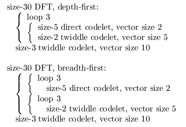
Fig. 10.5.1 Two possible decompositions for a size-30 DFT, both for the arbitrary choice of DIT radices 3 then 2 then 5, and prime-size codelets. Items grouped by a "{ " result from the plan for a single sub-problem. In the depth-first case, the vector rank was reduced to zero as per Plans for higher vector ranks before decomposing sub-problems, and vice-versa in the breadth-first case

As discussed previously in sections Review of the Cooley-Tukey FFT and Understanding FFTs with an ideal cache, the same Cooley-Tukey decomposition can be executed in either traditional breadth-first order or in recursive depth-first order, where the latter has some theoretical cache advantages. FFTW is explicitly recursive, and thus it can naturally employ a depth-first order. Because its sub-problems contain a vector loop that can be executed in a variety of orders, however, FFTW can also employ breadth-first traversal. In particular, a 1d algorithm resembling the traditional breadth-first Cooley-Tukey would result from applying Cooley-Tukey plans to completely factorize the problem size before applying the loop rule Plans for higher vector ranks to reduce the vector ranks, whereas depth-first traversal would result from applying the loop rule before factorizing each subtransform. These two possibilities are illustrated by an example in Fig. 10.5.1 above.

Another example of the effect of loop reordering is a style of plan that we sometimes call vector recursion (unrelated to “vector-radix” FFTs). The basic idea is that, if one has a loop (vector-rank 1) of transforms, where the vector stride is smaller than the transform size, it is advantageous to push the loop towards the leaves of the transform decomposition, while otherwise maintaining recursive depth-first ordering, rather than looping “outside” the transform; i.e., apply the usual FFT to “vectors” rather than numbers. Limited forms of this idea have appeared for computing multiple FFTs on vector processors (where the loop in question maps directly to a hardware vector). For example, Cooley-Tukey produces a unit input-stride vector loop at the top-level DIT decomposition, but with a large output stride; this difference in strides makes it non-obvious whether vector recursion is advantageous for the sub-problem, but for large transforms we often observe the planner to choose this possibility.

In-place 1d transforms (with no separate bit reversal pass) can be obtained as follows by a combination DIT and DIF plans Cooley-Tukey plans with transposes "Rank-0 plans". First, the transform is decomposed via a radix-$p$ DIT plan into a vector of $p$ transforms of size $qm$, then these are decomposed in turn by a radix-$q$, DIF plan into a vector (rank 2) of $p\times q$ transforms of size $m$. These transforms of size $m$ have input and output at different places/strides in the original array, and so cannot be solved independently. Instead, an indirect plan "Indirect plans" is used to express the sub-problem as $p q " role="presentation" style="position:relative;" tabindex="0">$

The FFTW planner

Given a problem and a set of possible plans, the basic principle behind the FFTW planner is straightforward: construct a plan for each applicable algorithmic step, time the execution of these plans, and select the fastest one. Each algorithmic step may break the problem into subproblems, and the fastest plan for each subproblem is constructed in the same way. These timing measurements can either be performed at runtime, or alternatively the plans for a given set of sizes can be precomputed and loaded at a later time.

$n$ increases. In order to reduce the planning time to a manageable level, we employ several heuristics to reduce the space of possible plans that must be compared. The most important of these heuristics is dynamic programmin: it optimizes each sub-problem locally, independently of the larger context (so that the “best” plan for a given sub-problem is re-used whenever that sub-problem is encountered). Dynamic programming is not guaranteed to find the fastest plan, because the performance of plans is context-dependent on real machines (e.g., the contents of the cache depend on the preceding computations); however, this approximation works reasonably well in practice and greatly reduces the planning time. Other approximations, such as restrictions on the types of loop-reorderings that are considered Plans for higher vector ranks are also described.

Alternatively, there is an estimate mode that performs no timing measurements whatsoever, but instead minimizes a heuristic cost function. This can reduce the planner time by several orders of magnitude, but with a significant penalty observed in plan efficiency; e.g., a penalty of 20% is typical for moderate $n\underset{\sim }{< }2^{13}$, whereas a factor of 2–3 can be suffered for large $n ≳ 216 " role="presentation" style="position:relative;" tabindex="0">$

Search

Text Color

Text Size

Margin Size

Font Type

DFT problem examples

The space of plans in FFTW

Rank-0 plans

Rank-1 plans

Direct plans

Cooley-Tukey plans

Plans for higher vector ranks

Indirect plans

Plans for prime sizes

Discussion

The FFTW planner

The problem to be solved

nn" role="presentation" style="position:relative;" tabindex="0">Contributor