3.8.2: Discrete Cosine Transformation
- Page ID
- 50953

In the language of linear algebra, the formula
\[\mathbb{Y} = \mathbb{C}\mathbb{X}\mathbb{D} \tag{3.10}\]
represents a transformation of the matrix \(\mathbb{X}\) into a matrix of coefficients \(\mathbb{Y}\). Assuming that the transformation matrices \(\mathbb{C}\) and \(\mathbb{D}\) have inverses \(\mathbb{C}^{−1}\) and \(\mathbb{D}^{−1}\) respectively, the original matrix can be reconstructed from the coefficients by the reverse transformation:
\[ \mathbb{X} = \mathbb{C}^{-1}\mathbb{Y}\mathbb{D}^{-1}. \tag{3.11}\]
This interpretation of \(\mathbb{Y}\) as coefficients useful for the reconstruction of \(\mathbb{X}\) is especially useful for the Discrete Cosine Transformation.
The Discrete Cosine Transformation is a Discrete Linear Transformation of the type discussed above
\[\mathbb{Y} = \mathbb{C}^{T}\mathbb{X}\mathbb{C}\tag{3.12}\]
where the matrices are all of size \(N×N\) and the two transformation matrices are transposes of each other. The transformation is called the Cosine transformation because the matrix \(\mathbb{C}\) is defined as
\[\tag{3.13} {\mathbb{C}}_{m,n} = k_n \cos \begin{bmatrix} \dfrac{(2m + 1)n\pi}{2N} \end{bmatrix} \text{where } k_n = \begin{cases} \sqrt{1/N} & \mbox{if }n = 0 \\ \sqrt{2/N} & \mbox{if otherwise} \end{cases} \]
where \(m, n = 0, 1, . . .(N − 1)\). This matrix \(\mathbb{C}\) has an inverse which is equal to its transpose:
\[\tag{3.14} \mathbb{C}^{-1} = \mathbb{C}.\]
Using Equation 3.12 with \(\mathbb{C}\) as defined in Equation 3.13, we can compute the DCT \(\mathbb{Y}\) of any matrix \(\mathbb{X}\), where the matrix \(\mathbb{X}\) may represent the pixels of a given image. In the context of the DCT, the inverse procedure outlined in equation 3.11 is called the Inverse Discrete Cosine Transformation (IDCT):
\[\tag{3.15} \mathbb{X} = \mathbb{C}\mathbb{Y}\mathbb{C}^T.\]
With this equation, we can compute the set of base matrices of the DCT, that is: the set of matrices to which each of the elements of \(\mathbb{Y}\) corresponds via the DCT. Let us construct the set of all possible images with a single non-zero pixel each. These images will represent the individual coefficients of the matrix \(\mathbb{Y}\). Figure 3.7(a) shows the set for 4×4 pixel images. Figure 3.7(b) shows the result of applying the IDCT to the images in Figure 3.7(a). The set of images in Figure 3.7(b) are called basis because the DCT of any of them will yield a matrix \(\mathbb{Y}\) that has a single non-zero coefficient, and thus they represent the base images in which the DCT “decomposes” any input image.
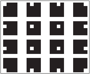
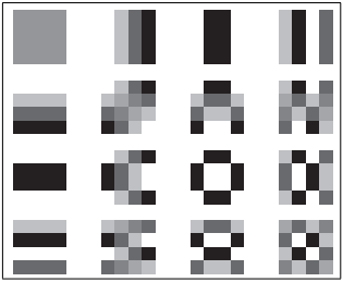
Figure 3.7: (a) 4×4 pixel images representing the coefficients appearing in the matrix \(\mathbb{Y}\) from equation 3.15. And, (b) corresponding Inverse Discrete Cosine Transformations, these ICDTs can be interpreted as a the base images that correspond to the coefficients of \(\mathbb{Y}\).
Recalling our overview of Discrete Linear Transformations above, should we want to recover an image \(\mathbb{X}\) from its DCT \(\mathbb{Y}\) we would just take each element of Y and multiply it by the corresponding matrix from 3.7(b). Indeed, Figure 3.7(b) introduces a very remarkable property of the DCT basis: it encodes spatial frequency. Compression can be achieved by ignoring those spatial frequencies that have smaller DCT coefficients. Think about the image of a chessboard—it has a high spatial frequency component, and almost all of the low frequency components can be removed. Conversely, blurred images tend to have fewer higher spatial frequency components, and then high frequency components, lower right in the Figure 3.7(b), can be set to zero as an “acceptable approximation”. This is the principle for irreversible compression behind JPEG.
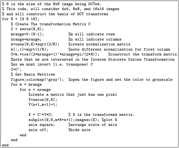
Figure 3.8 shows MATLAB code to generate the basis images as shown above for the 4×4, 8×8, and 16×16 DCT.